M  A  S  I

M A N A G E R I A L R A T I O S

by

H A N S J E S S E N

The Technical University of Denmark

November 1982

AMT Publication DI.82.85-A

.

ABSTRACT

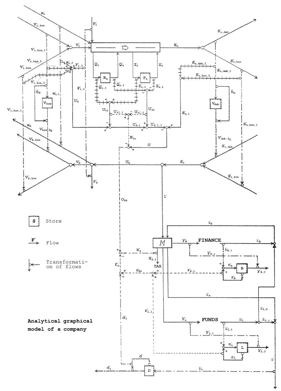
In order to determine managerial ratios as mathematical analytical functions of time there has been developed a graphical model of a firm. This model shows the physical relationship between fundamental principles of bookkee- ping, operating statements and managerial economics. The model is the structural basis of the determination of the mathematical analytical functions for management.

The analytical background of traditional ratio techniqu- es, including, Bela Gold lit. 40 and the Dupont pyramid, is described by means of a new developed general manage-rial ratio funktion.

.

- I -

CONTENTS

Page

Sumary V

Preface VI

Part A:

CHAPTER A

1. An analytical business model 1

1.1. Introduction 1

1.1.1. S. Eilon's model 1

1.1.1.1. Functional relationships and assumptions 3

1.1.1.1.1. Change in the cost structure 7

1.1.1.1.2. Change in the earnings structure 13

1.1.2. Assessment of S. Eilon's model 18

Part B:

CHAPTER_B

2. An analytical graphical business model 20

2.1. Activity parameters 20

2.1.1. Sales 20

2.1.2. Purchases 20

2.1.3. Inventories 22

2.2. Payment parameters, operations

2.2.1. Sales 22

2.2.2. Purchases 23

2.3. Market parameters, sales 23

2.3.1. Cash sales ratio q 23

2.3.2. The price p 24

2.3.3. Debit time d_D 24

2.4. Market parameters, purchases 25

2.4.l. Cash purchases ratio e 25

2.4.2. The price q₁ of raw materials 26

2.4.3. The price q₂ of labor hours 26

2.4.4 Credit time d_K 27

- II -

3.1. Income statement 28

3.1.1. Sales of goods 28

3.1.2. Costs 29

3.1.2.1. Inventories, additions (with signs) 30

3.1.3. Resource consumption (incl. F'_i,1) 33

3.1.4. Operating profit (before interest and deprec.) 33

3.1.5. Operating profit incl. inventory deprec. 33

4.1. Chanqe in liquidity (operations) 35

5.1. Cash balance 36

5.2. Bank loans 36

5.3. Loans (long-term) 37

6.1. Investment (in fixed capital) 38

7.1. Depreciation (for tax purposes) 39

8.1. Interest (for tax purposes) 40

9.1. Tax pavments 4O

10.1. Principal ratios 41

10.1.1. Operating profit 0^'(t) 41

10.1.2. Change in liquidity l^'(t) 42

10.1.3. Working capital K(t) 43

10.1.4. Contribution ratio DG(t) 43

10.1.5. Depreciation 44

10.1.6. Interest r^'_BL(t) 44

.

- III -

CHAPTER C

11. An analytical mathematical businessmodel 45

11.1. Physical and financial functions i the operating

system 45

11.1.1. Sales 45

11.1.2. Inventories 46

11.1.3. Output 50

l1.1.4. Sales, ingoing payments 50

11.1.5. Purchases, outgoing payments 51

11.1.6. Change in liquidity 52

11.2. Capital tied up in the operating system 52

11.2.1. Trade accounts receivable 52

11.2.2. Trade accounts payable 53

11.2.3. Raw materials invefitory 53

11.2.4. Finished goods inventory 54

11.2.5. Working capital (tied up in the operating system 54

12.1. Operatinq profit (for accountinq purposes) 55

12.2. Operating profit (computed on the basis of Fig. 2.1.) 56

12.2.1. Operating profit incl. inventory depreciation 58

12.3.1. Bank loans 59

12.3.2. Loans (long term) 60

12.3.3. Investments 60

12.4.1. Interest payments 61

12.4.2. Depreciation 61

12.4.3. Tax payments 61

12.4.4. Cash flow released 62

12.4.4.1. Interest relative 63

12.4.4.2. Depreciation relative 63

.

- IV -

13.1. Traditional ratios 64

13.1.1 Contribution ratio 64

13.1.2. Profit ratio 64

13.1.3. Break-even sales 64

13.1.4. Margin of safety 65

13.1.5. Applications, examples 65

13.2. Dupont pyramid 66

13.2.1 Ratio mathematics, general 68

CONCLUSION 7O

BIBLIOGRAPHY 72

.

- V -

SUMMARY

For the determination of ratios as analytical mathematical functions of time a graphical model of a firm has been developed. This model is a graphical representation of the relationships between fundamental aspects of the firm relating to book-keeping (records), accounting and managerial economics. The model forms the basis of the following deve- lopment of analytical mathematical functions. The mathematical back-ground of traditional ratio techniques, including Bela Gold lit. 40 and the Dupont pyramid, is shown through the development of a general ratio function.

Lyngby, November 1982

.

- VI -

PREFACE

The existing literature on accountancy and managerial economics has ma- de several attempts to improve the theoretical basis in order to provide management with a better understanding of business management possibili- ties.

In lit. 20, Albert Danielsson is dealing solely with purely analytical

aspects in relation to costs of production, and he has in that connec- tion developed symbolic flow charts for analysis purposes. This work seems to be of a very special character and not suited for overall ma- nagement purposes where the firm is to be seen as a whole. Links to inventories and the market are, for instance, missing.

Bela Gold, lit. 40, attempts to generalise accounting ratios in a tech-nical structure which includes managerial ratios. This technique seems to be very practicable but only for partial global business analyses. In this thesis a theoretical analysis of general ratios will be made, in-cluding the Dupont pyramid and including, in particular, Bela Gold's ratio technique.

J. W. Forrester, lit. 37, provides with his special representation

technique based on computer technology an excellent basis for analy- sing company behavlour. It gives, in a certain degree, a good insight into the behavlour of a firm in situations with different external and internal influences. Also here a fundamental mathematical model for purely analytical purposes is missing.

Dan Ahlmark, lit. 1, stresses the necessity of developing an analysis

model of the business which makes it possible to consider the current

integrated process, production, investment, financing activities of the business. To illustrate this need, an extensive empirical business ana- lysis is made, using generally known simulation techniques.

.

- VII -

Finn C. Sørensen, lit. 97, finds in his review of traditional accoun-

ting methods that a model should be developed for man agement which is

suitable for illustrating general matters in the firm, i.e. form the

basis of an actual managerial audit. By this is meant an examination of activities and matters underlying the financial/accounting report.

Samuel Eilon, lit. 30, attempts with his mathematical model to compute

the rate of return as a function of general business parameters, using, among other things, a symbolic graphical representation technique to de-scribe the inter relationships of the equations. This work seems to be the most interesting work in the literature seen in relation to the de- velopment of a generalised business analysis model.

Using the literature reviewed as a starting point with special impor-

tance being attached to the above authors, the structure and field of

applications of Eilon's model in lit. 30 will be analysed in detail.

After this analysis, a graphical analytical business model is developed in Chapter B including book keeping, accounting and financial concepts to be employed by the business management. Using this model it is possi-ble to carry out an actual managerial audit as described by Finn C. Sø- rensen, among others.

Chapter C defines an analytical mathematical business model based on the general graphical structure shown in Chapter B. As a special starting point is taken the fact that any sales curve may be composed of a piece- wise linear function. The basic element of the sales function is thus chosen as a linear function of time.

Based on the developed mathematical functions the most common accounting ratios are computed as a function of time.

.

- VIII -

Bela Gold's ratio technique is examined more ciosely, using general ma-thematical ratio functions developed in this report, and an attempt is made to explain it by means of these functions, which are also used to illustrate the technical background of the computation of the rate of return in the Dupont pyramid.

.

C H A P T E R A

.

- 1 -

1. An analytical business model

1.1. Introduction

During the mentioned review of the litterature only one source was found, which was suitable for forming the basis of the development of

the general mathematical business model in Chapters B and C. This sour- ce was Samuel Eilon's article in OMEGA 1997, Vol. 5, No. 6: "A Profita- bility Model for Tactical Planning", lit. 30.

In the following the mentioned article will therefore be discussed as

an introduction to the analytical mathematical business model in Chap-

ter C.

1.1.1 S. Eilon's model

The article starts by pointing out that simple models reflecting aggre- gate company behaviour in response to changes imposed by management de- cisions and/or outside factors provide useful tools for management for tactical planning purposes.

As his starting point, Eilon takes the rate of return r expressed as:

(p - c)V

r = ¾¾¾¾¾ (1)

I

or

earnings

r = ¾¾¾¾¾¾¾¾¾¾¾ (2)

total investment

where

.

- 2 -

p = unit price per unit of output

c = unit cost per unit of output

V = output units per time unit

I = total investment

Attention is drawn to the fact that for macro economic purposes it is

possible to compute the ratio r from the definition equation (2) and

thus obtain information on an industry's "profitability".

Equation (1) is a micro economic rewriting of (2) based on "logical"

considerations. The numerator in equation (1) is fairly well defined,

also in a micro economic model, but the denominator I, total assets,

which serves the main purpose, is difficult to determine in practice.

Additions to and disposals of assets as well as changes in the market

value of these assets take place currently.

The practical purpose of the computation of the rate of return is a

desire to obtain an equivalent measure of the return on investment. It

appears from the above that in practice the com putation of r involves

great uncertainty so that r is a relatively uncertain measure of profi- tability. If the following definitions are now introduced

dp dc dI

p^* = ¾¾¾ ; c^* = ¾¾¾ ; I^* = ¾¾¾ ,

p d I

where the changes dp, dc, dV and dI are given, equation (1) can be

transformed into

1 1 + V^*

r^* = ¾¾¾¾¾¾ (¾¾¾¾¾ (p^* - (1 - a) c^*) + V^* - I^*) (3)

1 + I^* a

.

- 3 -

p - c

given definition a = ¾¾¾¾¾ = the relative profit margin.

p

As regards equation (3), S. Eilon observes that it is an analytical tool for assessing the effects on r of changes of the variables of the

right hand side.

In practice, a functional inter relationship exists very often between

these variables; a later change in the selling price or the cost price will, for instance, bring about changes not only in investments (in

the working capital) but also in demand and hence output.

1.1.1.1. Functional relationships and assumptions

Eilon assigns to the cost c per output unit the following conventional

functional expression:

F J

c = s + ¾¾ + ¾¾ (4)

V V

where

s represents direct unit costs

F

¾¾ represents indiret unit costs excl. interest

V

J

¾¾ represents interest charge per unit.

V

Equation (4) is a so called traditional economic calculation of total

unit costs. It should, however, be noted that from a general accoun-

ting point of view there is no real justification for equation (4). It

is simply an appropriate formula for the unit cost function in relati-

on to the traditional theory of managerial economics, which makes it

possible to carry out simple partial operations research computations

.

- 4 -

concerning, for instance, profit maximization in relation to various

alter natives.

The stressing of the point that equation (4) has no real physical ju-

stification is due to the fact that equation (4) is a simple transfor- mation of equations (5) and (6).

TO = c V (5)

TO = s V + F + J (6)

Equation (5) is here a purely non physical definition equation (addi-

tion of simple "krone amounts") for the total costs TO specified via

the definition equation (6). It will be seen that these definition equa- tions give rise to problems in connection with the physical interpreta- tion. What is, for instance, meant by fixed costs, and how are they de- fned in relation to, say, the interest charges J ?

A transformation of equation (4) using the definitions s = f₁ c , F/V

= f₂ c and J/V = f₃ c gives

1

c^* = f₁ s^* + ¾¾¾¾¾(f₂ F^* + f₃ J^* - (1 - f₁) V^*) (7)

1 + V^*

This equation (7) shows that with a good approximation we have:

c^* = f₁ s^* + f₂ F^* + f₃ J^* - (1 - f₁) V^* (8)

Interpretation of the contents of, for example, (8) will show that the

percentage change of the unit costs is equal to the weighted sum of the percentage change of s, F, J and V.

.

- 5 -

Concerning investments I, S. Eilon assumes:

I_W = A + B (9)

I = I_W + I_F (10)

where

I_W = the working capital

I_F = investment in fixed assets

B = bank loans + overdrafts

A = other loans

S. Eilon also defines:

w = I_W/I (10a)

l = B/I_W (10b)

J = j B , where j is the interest rate (lOc)

Equation (10) can now be transformed into:

I^* = w I^*_W + (1 - w)I^*_F (11)

Equation (9) can be transformed into:

I^*_W = (1 - l) A^* + l B^* (12)

A combination of equation (12) and equation (11) will take the form:

I^* = w ((1 - l) A^* + l B^*) + (1 - w) I^*_F (13)

For use in the actual planning process of the business, S. Eilon assu-

mes that

.

- 6 -

I^*_F = 0 (14)

and

A^* = 0 (15)

It is also assumed that w and l are constant (the artiticle does not

mention this explicitly).

Based on the mentioned assumptions equations (12) and (13) are then

reduced to

I^*_W = l B^* (16)

and

I^* = w l B^* (17)

gives the conditions (14) and (15).

In connection with the determination of changes in the working capital

I_W, S. Eilon writes:

"No single relationship between working capital and the 1evel of ac-

tivity in the firm is universally accepted and we may proceed to ex-

plore two possible assumptions."

These two assumptions are combined as a linear combination

I^*_W = g (p v)^* + h(c V)^* (18)

which denotes that the working capital (tied up in the operating sy-

stem is changed as a linear combination of the change in sales and the

change in cost. S. Eilon claims that no controller has difficulty in

determining empirically the constants g and h. It must therefore be

.

- 7 -

possible to find a physical model which describes these empirical facts. A mathematical analytical solution to this problem is described

in Chapter C.

S. Eilon proceeds to consider three cases which are relevant for tac-

tical planning purposes:

1. Change of s, F and j

2. Change of V

3. Change of p

In the first case changes in the cost structure are considered. The

following two cases deal with changes in sales and changes in the mar-

ket price, i.e. two situations where the earnings structure is chan-

ged. However, as regards cases 2 and 3, it is natural to describe them

together as will be seen later. The things to be discussed are therefo- re as follows:

1. Change in the cost structure caused by changes in s, F and j.

2. Change in the earnings structure caused by changes in V given the

market elasticity e.

1.1.1.1.1. Change in the cost structure

Attention is drawn to the fact that in his case 1 S. Eilon discusses

an iterative process, physical and mathematical, in connection with the final computation of c^*. From a physical point of view, this is in full accordance with the accounting theory, as will be shown later in the ge- neral mathematical business model. S. Eilon attempts to provide this "fact" of the expressions de scribed here through the mathematical convergence in the computation of total unit costs as shown in the article. In this respect, however, it does not seem to be a good idea to combine physical and mathematical facts too much since, as has already been

- 8 -

mentioned, S. Eilon employs a non physical definition of unit costs (see equation (4), which highly weakens the foundation of Eilon's conclusi- ons.

S. Eilon elaborates on this definiton of the unit cost, one of the prin- ciples of traditional theories of managerial economics, in case 1. It is exactly these conflicts between the physical conditions in the firm and the traditional theory of managerial economics which have caused the de- velopment of the mathematical business model described in Chapter C.

With a view to solving the existing mathematical problem, equation

(1Oc) is transformed into:

J^* = j^* + (1 + j^*) B^* (2o)

The mathematical problem can now be solved by means of the followinq

previously shown equations (7), (16) and (18) together with the reated conditions:

Equations:

1

c^* = f₁ s^* + ¾¾¾¾ (f₂ F^* + f₃ J^* - (1 - f₁) V^*) (21)

1 + V^*

J^* = j^* + (1 + j^*) B^* (22)

I^*_W = l B^* (23)

I^*_W = g(p v)^* + h(c v)^* (24)

.

- 9 -

given the conditions

V^* = 0 (25)

p^* = 0 (26)

A solution is obtained as follows:

From equation (24) with the conditions (25) and (26) it follows that

I^*_W = h c^* (27)

Equation (27) and (23) give

h

B^* = ¾¾ c^* (28)

l

A combination of equation (28) and (22) gives

h

J^* = j^* + (1 + j^*) ¾¾ c^* (29)

l

A combination of equation (29) and (21) gives

f₁ s^* + f₂ F^* + f₃ j^*

c^* = ¾¾¾¾¾¾¾¾¾¾¾¾¾¾ (30)

h

1 - (1 + j^*) ¾¾ f₃

l

In equation (30) the question is raised whether

h

(1 + j^*) ¾¾ f₃ < 1

l

has been satisfied as, in practice, equation (lOb) shows that

1 I_W

¾¾ = ¾¾

l B

.

- l0 -

Normally will I_W < B, hence

1

¾¾ < 1

l

As typically in practice h < 1, f₃ < 0.5 and (1 + j^*) < 1.5, inequa1ity

(31) gives

h 1

(1 + j^*) ¾¾ f₃ < 1,2 ¾¾ 0.5

l 1

or

h

(1 + j^*) ¾¾ f₃ < 0.6

l

From this will be seen that, in practice, inequality (31) has been sa-

tisfied.

S. Eilon introduces a new ratio H = I_W /(c V) for the purpose showing

that inequality (31) has been satisfied in practice. This seems to be

a purely mathematical exercise without any relevant justification phy-

sically. It is once more pointed out that S. Eilon overinterprets the

mathematical consequences of the use of the equation (4) defined on the basis of managerial economics.

For the purpose of computing the rate of return the equations (3),

(lOa) and (18) are used to solve the equations:

1 1 + V^*

r^* = ¾¾¾¾¾ (¾¾¾¾¾(p^* - (1 - a) c^*) + V^* - I^*) (32)

1 + I^* a

1

I = ¾¾ I_W (33)

w

.

- 11 -

I^*_W = g(p V)^* + h(c v)^* (34)

with the conditions:

f₁ s^* + f₂ F^* + f₃ j^*

c^* = ¾¾¾¾¾¾¾¾¾¾¾¾¾¾ (35)

h

1 - (1 + j^*) ¾¾ f₃

l

V^* = 0 (36)

p^* = 0 (37)

Equation (34) gives, cf. equation (27)

I^*_W = h c^* (38)

Equation (33) is transformed into

I^* = w I^*_W (39)

Equatioin (38) combined with equation (39) gives

I^* = w h c^* (40)

Equation (32) gives with equation (40) and the conditions (35),

(36) and (37) the following expression

c* 1 - a

r^* = - ¾¾¾¾¾¾¾¾ (¾¾¾¾¾ h w ) (41)

1 + w h c^* a

given

f₁ s^* + f₂ F^* + f₃ j^*

c^* = ¾¾¾¾¾¾¾¾¾¾¾¾¾¾ (30)

h

1 - (1 + j^*) ¾¾ f₃

l

.

- 12 -

As regards equation (30) it should be noted that S. Eilon finds it

"justified" to define a quantity

c^*₀ = f₁ s^* + f₂ F^* + f₃ j^* (42)

as unit costs, if h = 0, i.e. if no changes occur in the working ca-

pital with the given conditions V^* = O and p^* = 0 , cf. equa tion (38).

Equation (35) now takes the form

c^*₀

c^* = ¾¾¾¾¾¾¾¾¾¾¾¾¾¾ (30)

h

1 - (1 + j^*) ¾¾ f₃

l

given

c^*₀ = f₁ s^* + f₂ F^* + f₃ j^*

Further, on the basis of the denominator in equation (43), S. Eilon

defines a ratio u as he seems to find it desirabie that all ratios oc-

cur in product form. For instance, as mentioned previously in this

connection, he also defines the ratio H = I_W/(c V), which from the

point of view of accounting theory is a very specific concept.

A look at equation (43) will show that it takes the form of "ratios",

i.e. it contains dimensionless quantities, which are all ratios in the

firm. Therefore, it does not seem to be a very desirable measure to

introduce further ratios to give the equa tion a changed algebraic

structure.

However, for analytical purposes in connection with an analysis of the

numerical "behaviour" of equation (43) it may be useful to define a

parameter x given by

.

- 13 -

h

x = (1 + j^*) ¾¾ f₃ (44)

l

so that equation (43) is transformed into

c^*₀

c^* = ¾¾¾¾¾ (45)

1 - x

given

h

x = (1 + j^*) ¾¾ f₃ (46)

l

and

c^*₀ = f₁ s^* + f₂ F^* + f₃ j^* (47)

Thus, by a preliminary nurnerical analysis of (45), x may be a11owed

to vary in the interval 0 < x < 1. It should be noted that x is here a

parameter. In the second phase of such an anal ysis a numerical ana- lysis of equation (46) can be carried out, given certain selected va- lues of x.

1.1.2.1.2. Change in the earnings structure

In this case where management wishes to consider the influence of the

market on the rate of return, etc., the following expression is assu-

med to apply

V^* = - e p^* (48)

given p^*.

.

- 14 -

The problem is thus given by the equations

1

c^* = f₁ s^* + ¾¾¾¾¾ (f₂ F^* + f₃ J^* - (1 - f₁) V^*) (49)

1 + V^*

J^* = j^* + (1 + j^*) l B^* (50)

I^*_W = l B^* (51)

I^* = g(p V)^* + h(c V)^* (52)

with the conditions:

s^* = 0 (53)

F^* = 0 (54)

j^* = 0 (55)

V^* = - e p^* (56)

Here equation (52) is transformed into

I^*_W = (g + h)V^* + (g p^* + h c^*)(1 + V^*) (56a)

After the transformation of the above equations and with the above

conditions the following equations are developed:

1

c* = ¾¾¾¾¾ (f₃ B^* - (1 - f₁) V^*) (57)

1 + V^*

1

B* = ¾¾((g + h) V^* + (g p^* + h c^*)(1 + V^*)) (58)

l

given the condition V^* = - e p^* (59)

.

- 15 -

Now equations (57), (58) and (59) give by simple reduction

e p^* 1 f₃

c^* = (1 - f₁) ¾¾¾¾¾ ¾¾¾¾¾¾¾¾¾¾ (1 - ¾¾¾¾¾¾¾

1 - e p^* f₃ (1 - f₁) l

1 - ¾¾¾ h

l

(h + g(1 + p^* - e^-1))) (60)

given the conditions

s^* = 0 (61)

F^* = 0 (62)

j^* = 0 (63)

V^* = - e p^* (64)

In connection with the practical use of equation (60) it might be de-

sirable to define a change in the unit cost cx* given by

e p^*

c^*_x = (1 - f₁) ¾¾¾¾¾¾ (65)

1 - e p^*

which has been obtained by putting s^* = 0, F^* = 0 and J^* = 0 in equati- on (7). c^*_x can here be interpreted as the change in the unit cost if the only thing to be considered is a change in the price p.

Moreover, from equation (60) can be defined

g

y = ¾¾¾

h

which may be interpreted as the need of investment in the working ca-

pital caused by sales in relation to caused by costs (see equation (18)).

.

- 16 -

The system of equations (60) .... (64) is now given the form

c^*_x x

c* = ¾¾¾¾ (1 - ¾¾¾¾ (1 + y(1 + p^* - e^-1))) (66)

1 - x 1 - f₁

given the conditions

h

x = (1 + j^*) ¾¾ f₃ (67)

l

g

y = ¾¾¾

h

Using equations (3), (17), (57) and (60) .... (64) the following sy -

stem of equations can now be defined for the determination of the rate

of return.

Equation:

1 1 - e p^*

r^* = ¾¾¾¾¾¾¾ (¾¾¾¾¾¾ (p^* - (1 - a) c^*) - e p^* - w I^*_W) (69)

1 + w I^*_W a

given the conditions

s^* = 0 (70)

F^* = 0 (71)

j^* = 0 (72)

V^* = - e p^* (73)

I^*_W = (g + h)V^* + (g p^* + h c^*)(1 + V^*) (74)

e p^* 1 f₃

c^* = (1 - f₁) ¾¾¾¾¾ ¾¾¾¾¾¾¾¾¾¾ (1 - ¾¾¾¾¾¾¾

1 - e p^* f₃ (1 - f₁) l

1 - ¾¾¾ h

l

(h + g(1 + p^* - e^-1))) (75)

.

- 17 -

If changes are recorded only in V, the following system of equations

is obtained by replacing p^* with V^* and putting p^* = 0 and e^-1 = 0 in

the above equations:

V^* 1 f₃

c^* = - (1 - f₁) ¾¾¾¾¾ ¾¾¾¾¾¾¾¾¾¾ (1 - ¾¾¾¾¾¾¾

1 - V^* f₃ (1 - f₁) l

1 - ¾¾¾ h

l

(h + g)) (76)

given the conditions

s^* = 0 (77)

F^* = 0 (78)

j^* = 0 (79)

e^-1 = 0 (80)

p^* = 0 (81)

and the system of equations:

1 1 - a

r^* = ¾¾¾¾¾¾¾ (V^* - ¾¾¾¾¾ (1 + V^*) c^* + w I^*_W) (82)

1 + w I^*_W a

given the conditions

s^* = 0 (83)

F^* = 0 (84)

j^* = 0 (85)

I^*_W = (g + h(1 + c^*)) V^* + h c^* (86)

V^* 1 f₃

c^* = - (1 - f₁) ¾¾¾¾¾ ¾¾¾¾¾¾¾¾¾¾ (1 - ¾¾¾¾¾¾¾

1 - V^* f₃ (1 - f₁) l

1 - ¾¾¾ h

l

(h + g)) (87)

Attention is called to the fact that the resuits in this Chapter dif-

fer from S. Eilon's results in cases 2 and 3. The following Chapter

will indude a general discussion of S. Eilon's results and models in

the light of the results achieved here.

- 18 -

1.1.2. Assesment of S. Eilon's model

It has already been pointed out that the basis of S. Eilon's model gi- ves rise to the question as to whether it serves any purpose to carry out these computations and at the same time attach such fundamental importance to the models shown in the article in relation to the phy- sical business situation.

Thus, S. Eilon assumes that eguation (4) is fundamental, i.e. a funda- mental starting point for considerations based on managerial economies. With reference to eguations (5) and (6) it was stated that this is a point of view which should be examined more closely. This examination leads to the point that eguation (4) is a purely mathematical definition equation, i.e. an equation which is not founded on real physical facts (equation (6)'s right hand side consists of a sum of elements of widely differing physical origin with only one thing in

common: the value "DKK").

Owing to the mathematical structure of equation (4) it will mathema-

d J(V)

tically be convergent as where U £ ¾¾¾ (¾¾¾) £ K , in practice U

dV V

and K are constants. The physical convergence also exists in connec- tion with the changes in the tactical planning process (transients) under consideration. It should be noted that the mathematical model shows the relationships between changes in states" (i.e. time is not included explicitly) with the related mathematical characteristics of the manner of converging. The physical activity/cash flow model of the business is knovn also in practice to possess convergent characteri- stics as a function of time. See chapter C.

Against this background it is important not to attach too great impor-

tance here to the applicability of S. Eilon's model to an interpreta-

tion of the dynamics of the firm (for tactical planning purposes).

Thus, the mathematical business model, Chapter C, is not to take state

functions as its starting point but only use a time description of the

functions.

.

- 19 -

The graphical description used by S. Eilon can only be regarded as a

dear description of the equations between the individual variable.

being studied.

In Chapter B a physical model description of the business will the-

refore be given first, the greatest importance being attached to ma-

king the physical/financial description as realistic as possible. Af-

ter this the mathematical déscription is developed in Chapter C.

The results achieved in the present Chapter A differ from S. Eilon's

results as far as computations of the effects of changes in the ear-

nings structure are concerned. It is pointed out that S. Eilon's un-

structuralized consideration of the mathematical methods of solution

may be the reason for the deviating results in the article.

The central equation (18), which estimates the relationship between the working capital tied up in the operating system, will be analysed in detail in Chapter C.

.

C H A P T E R B

.

- 20 -

2. An analytical graphical business model

This Chapter describes an analytical graphical business model (see Fig. 2.1.). This model will form the basis of a mathematical analytical description of the business so that this description can be used by the business management for their principal planning activities. The model will integrate principal elements of managerial economics and the ac- counting theory, it being assumed that the business comprises an acti- vity/cash flow and related principal assets (accounts payable, accounts receivable, inventories). It is management's task to achieve the best possible composition of this general structure by using some of the ra- tios defined in the model.

2.1. Activity parameters

2.1.1. Sales

The volume of goods sold by the firm per unit is denoted with S^'_u. Sales are here divided into two main components of which one is the reference sales S^'_u,kon, which refers to the share of sales which is paid for in cash. The other component of sales is denoted with S^'_u,deb,which refers to the share of sales which is paid for by the trade accounts receivable the debit time deltaD after delivery from the firm. Here the following eguation applies:

S^'_u(t) = S^'_u,deb(t) + S^'_u,kon(t) (88)

2.1.2. Purchases

The firm is supplied with a number of labor hours per time unit a^'_i.

The firm is supplied with the volume of goods per time unit V^'_i. This flow of goods consists of two main components of which one is the refe- rence purchase V^'_i,kon, and the other the goods purchased on credit V^'_i,kre, which are paid for by the firm after the credit time d_K.

- 21 -

Figure 2.1

(Click on the figure for 200%)

.

- 22 -

The following equation applies:

V^'_i(t) = V^'_i,kre(t) + V^'_i,kon(t) (89)

The firm is supplied with the fixed volume of resources per time unit F^'_i. This flow of resources may, for example, include electricity, administration, heating, rent, etc.

2.1.3. Inventories

The volume of raw materials per time unit Q^'_i is added to the raw mate-

rials inventory consisting of the volume R_L. From the raw materials in- ventory is deduced the raw materials volume Q^'_u. The following equation

applies here:

t

R_L = ò (Q^'_i(t) - Q^'_u(t))dt (90)

0

The volume of finished goods per time unit Z^'_i is added to the finished

goods inventory consisting of the volume F_L. From the finished goods

inventory is deduced the finished goods volume Z^'_u. The following equa- tion applies here:

t

F_L = ò(Z^'_i(t) - Z^'_u(t))dt (91)

0

2.2. Payment parameters, operations

2.2.1. Sales

The total volume of means of payment per time unit from the customers is denoted with S^'_i. This payments flow consists of two components. One component is the payments flow S^'_i,kon stemming from the cash sales flow

S^'_u,kon. The other component S^'_i,deb is the payments flow stemming from the credit sales flow S^'_u,deb. Here the following equation applies:

S^'_i(t) = S^'_i,kon(t) + S^'_i,deb(t) (92)

.

- 23 -

2.2.2. Purchases

The total volume of means of payment per time unit for operations is denoted with U^'_b. This payments flow is composed of three components, a^'_b and V^'_b and F^'_b. a^'_b is the payments flow corresponding to the flow of hours consumed a^'_i, V^'_b is the payments flow corresponding to the flow of raw material purchases V^'_i, F^'_b is the payments flow corresponding to the flow of fixed resources consumed F^'_i. The following equation applies:

U^'_b(t) = a^'_b(t) + V^'_b(t) + F^'_b(t) (93)

The payments flow V^'_b is made up of two components. One component is the payments flow V^'_b,kon corresponding to the cash purchases of rawmaterials V^'_i,kon; the other component is the payments flow V^'_b,kre corresponding to the credit purchase of raw materials V^'_i,kre. The following equation applies:

V^'_b(t) = V^'_b,kon(t) + V^'_b,kre(t) (94)

2.3. Market parameters, sales

With a viev to depicting the fundamental financial effects of the mar- ket on the firm as well as its effects on earnings the market is cha- racterized by three basic components q , p and d_D. They also describe the fundamental link between the firm's sales of goods and the related payments flows.

2.3.1. Cash sales ratio q

The cash sales ratio is defined by the equation;

S^'_u,kon(t) = q S^'_u(t) (95)

where 0 £ q £ 1

In a manufacturing business q will typically be placed in the in- terval 0 £ q £ 0.2. In a supermarket q will typically be in the interval 0.8 £ q £ 1.

.

- 24 -

2.3.2. The price p

The price of the firm's product(s) is defined by the eguations

S^'_u,kon,1(t) = p S^'_u,kon(t) (96)

S^'_i,kon(t) = S^'_u,kon,1(t) (97)

where S^'_u,kon,1(t) is the flow of debts corresponding to the sales flow S^'_u,kon(t) (i.e. the current sending out of invoices stating the amount of debt; see equation (96)). Equation (97) expresses the fact that the flow of debts S^'_u,kon,1(t) is equal to the payments flow from the customers (cash payment).

In practice, it should be noted that there is normally only a tempora- ry time lag between invoicing and sales. However, it has a temporary negative effect on liquidity and the computation of results. Manage- ment will therefore as far as possible make sure that invoicing is done without the mentioned delays.

2.3.3. Debit time d_D

This model defines the debit time d_D as the time from the time of de- livery of the goods from the firm until the time of payment by the cu- stomer for the goods. In practice, d_D is spread over the individual cu- stomers but with well defined terms of payment the mean value can be adopted.

The definition of d_D can be expressed by the equations

S^'_u,deb,1(t) = p S^'_u,deb(t) (98)

V^'_deb,dD(t) = S^'_u,deb,1(t - d_D) (99)

S^'_i,deb(t) = V^'_deb,dD(t) (100)

.

- 25 -

S^'_u,deb,1 refers here to the invoice flow corresponding to the credit sales flow S^'_u,deb cf. equation (98). Equation (99) gives a funational description of a function V^'_deb,dD(t), which can be defined as the pay- ments flow (documents) corresponding to the actual receipt of payments S^'_i,deb(t) cf. equation (100). In practice, no time lag is found between the two last mentioned functions.

In pratice, attention should be paid to the fact that there may be a time lag in the business between invoicing and sales, the result being changes in liquidity and the computation of earnings. Management usu- ally aims at applying equation (98) in practice, i.e. no time lag.

2.4. Market parameters, purchases

With a view to depicting the fundamental financial effects of the pur- chasing market on the firm as well as its effects on costs, it is cha- racterized by four basic components epsilon, q₁, q₂ and d_K. They describe the fundamental link between the firm's purchases of resources and the related payments flows.

2.4.1. Cash purchases ratio e

The cash purchases ratio is defined by the equation:

V^'_i,kon(t) = e V^'_i(t) (101)

where 0 £ e £ 1

In, say, a manufacturing business e will typically be placed in the interval 0 £ e £ 0.2. This is also a typical feature in a trading firm.

2.4.2. The price q₁ of raw materials

The price of the firms raw materials is defined by the equation:

.

- 26 -

V^'_i,kon,1(t) = q₁ V^'_i,kon(t) (102)

V^'_b,kon(t) = V^'_i,kon,1(t) (103)

where V^'_i,kon,1(t) is the flow of debts corresponding to the raw materials flow V^'_i,kon(t) (i.e. the current receipt of invoices stating the amounts of debts); see equation (102). Equation (103) expresses the fact that the flow of debts V^'_i,kon,1(t) is equal to the payments flow to suppliers (cash payment).

In practice, attention should bepaid to the fact that the time lag between the supplier's invoicing and the supplies of raw materials is usually a temporary feature which has a temporary positive affect on liquidity and the computation of results.

2.4.3. The price q₂ of labor hours

The price of the firm's labor hours is defined by the equations

a^'_i,1(t) = q₂ a^'_i(t) (104)

a^'_b(t) = a^'_i,1(t) (105)

where a^'_i,1(t) is the time ticket flow corresponding to the flow of labor hours used a^'_i(t) (i.e. the current issuing of time tickets stating wages earned); see equation (17). Equation (18) expresses the fact that the time ticket flow a^'_i,1(t) is equal to the time rate flow a^'_b(t).

In practice there is a certain time lag between functions on the right hand side and the left hand side of the equal sign in equation (104). This time lag is ignored here. There is usually no time lag between

the functions of equation (105), or the time lag is relatively small and of no importance here.

.

- 27 -

2.4.4. Credit time d_K

This model defines the credit time d_K as the time from the time of de- livery of the raw materials to the firm until the time of payment by the firm for the raw materials. In practice, d_K is spread over the in- dividual suppliers but with well defined terms of payment the mean va- lue can be used. The definition of d_K can be expressed by the equati- ons:

V^'_i,kre,1(t) = q₁ V^'_i,kre(t) (106)

V^'_kre,dK(t) = V^'_i,kre,1(t - d_K) (107)

V^'_b,kre(t) = V^'_kre,dK(t) (108)

where V^'_i,kre,1(t) refers here to the invoice flow corresponding to the

credit purchases flow V^'_i,kre(t), cf. equation (106). Equation (107) gi-ves a functional description of a function V^'_kre,dK(t) which can be defined as the payment order flow (documents) corresponding to the actual effecting of payments V^'_b,kre(t), cf. equation (108). In practice, there is no time lag between the two last mentioned functions.

In practice, attention should be paid to the fact that the time lag between the supplier's invoicing and the supplies of raw materials is usually a temporary feature which has a temporary positive affect on liquidity and the computation of results.

The following equations are defined in relation to the fixed resources consumed F^'_i and the related fixed costs F^'_b.

F^'_i,1(t) = k F^'_i(t) (109)

F^'_b(t) = F^'_i,1(t) (110)

.

- 28 -

where F^'_i,1(t) in equation (109) refers to the flow of debts in the form of invoices (stating amounts) corresponding to the fixed resoures flow F^'_i(t). k denotes a symbolic operator in the form of an average price of the fixed resources unit. In practice, there is some time lag between the functions in eguation (110). As, however, the fixed costs by definition are constant in time, such a time lag is not important in this context.

3.1 Income statement

In this Chapter an income statement for operations is presented (be- fore depreciation, etc.) using the general main principles of accoun- ting theory.

3.1.1 Sales of goods

Sales of goods are defined on the basis of the following equations:

S^'_u,kon,2(t) = S^'_u,kon,1(t) (111)

S^'_u,deb,2(t) = S^'_u,deb,1(t) (112)

S^'_u,1(t) = S'_u,kon,2(t) + S^'_u,deb,2(t) (113)

Eguation (111) expresses the fact that the flow of debts (in the form of invoices with statement of amounts) S^'_u,kon,1(t) gives rise to an e- qually large information flow S^'_u,kon,2(t). This quantity is identital with the current crediting to the cash sales account.

From equation (112) follows that the flow of debts S^'_u,deb,1(t) causes an equally large information flow S^'_u,deb,2(t). This quantity is iden- tical to the current crediting to the credit sales account.

Total uales in the form of the information flow S^'_u,1(t) corresponding to the total crediting to the sales account are then obtained from e- quation (113).

.

- 29 -

3.1.2 Costs

The costs of the firm in connection with production and sales are de- fined by the following equations:

V^'_i,kon,2(t) = V^'_i,kon,1(t) (114)

V^'_i,kre,2(t) = V^'_i,kre,1(t) (115)

a^'_i,2(t) = a^'_i,1(t) (116)

F^'_i,2(t) = F^'_i,1(t) (117)

U^'_d(t) = V^'_i,kon,2(t) + V^'_i,kre,2(t) + a^'_i,2(t) + F^'_i,2(t) (118)

Equation (114) expresses the fact that the invoice flow from the cash purchase V^'_i,kon,1(t) is corrently debited to the cash purchases account

to the extent of the cash flow V^'_i,kon,2(t).

Equation (115) expresses the fact that the invoice flow from the cre- dit purchase V^'_i,kon,1(t) is currently debited to credit purchases account to the extent of the cash flow V^'_i,kre,2(t).

Equation (116) denotes the functional relationship between the time ticket flow a^'_i,1(t) and the current debiting to the time rate account of the wage payment flow a^'_i,2(t).

Equation (117) expresses the functional relationship between the in- voice flow F^'_i,1(t) for fixed costs and the current debiting of the cash flow F^'_i,2(t) to the fixed costs account.

The total cost flow is defined by equation (118).

.

- 30 -

3.1.2.1 Inventories, additions (with signs)

By way of introduction, it is mentioned that the signs relating to additions to inventories (as a mean time value) are assumed to be the same as those relating to additions to sales (as a mean time value). Against this background the additions to the individual inventories will for principal planning purposes have the same signs. The inventories only serve as "standby stores" in case of emergancy events" i.e. in normal operation state "the materials and products go directly through the factory. Thus, the following systems of equations apply:

Q^'_i(t) > 0

Q^'_u(t) = 0

d S^'_u

¾¾¾¾ > 0 Þ (119)

dt

Z^'_i(t) > 0

Z^'_u(t) = 0

Q^'_i(t) = 0

Q^'_u(t) = 0

d S^'_u

¾¾¾¾ = 0 Þ (120)

dt

Z^'_i(t) = 0

Z^'_u(t) = 0

Q^'_i(t) = 0

Q^'_u(t) > 0

d S^'_u

¾¾¾¾ < 0 Þ (121)

dt

Z^'_i(t) = 0

Z^'_u(t) > 0

.

- 31 -

The system of equations (119) denotes that inventories rise when sales rise.

The system of equations (120) denotes that inventories are constant when sales remain unchanqed.

The system of equations (121) denotes that inventories fall when sales fall.

Based on these main principles for the model the following equations can be developed.

Q^'_i,1(t) = q_R Q^'_i(t) (122)

Q^'_u,1(t) = q_R Q^'_u(t) (123)

Z^'_i,1(t) = q_F Q^'_i(t) (124)

Z^'_u,1(t) = q_F Z^'_u(t) (125)

U^'_tl(t) = Q^'_i,1(t) + Z^'_i,l(t) (126)

U^'_al(t) = Q^'_u,1(t) + Z^'_u,1(t) (127)

where Q^'_i,1(t) is the flow of additions to raw materials invento-

ries corresponding to the additions to rawmateri-

als inventory records with statement of amounts.

Q^'_u,1(t) is the flow of deductions to raw materials invento-

ries corresponding to the deductions to raw mate-

rials inventory records with statement of amounts.

Z^'_i,1(t) is the flow of additions to finished goods invento-

ries corresponding to the additions to finished

goods inventory records with statement of amounts.

.

- 32 -

Z^'_u,1(t) is the flow of deductions to finished goods inven-

inventories corresponding to the deductions to fi-

nished goods inventory records with statement of

amounts.

q_R denotes the caiculated rav material price per unit

of finished goods.

q_F denotes the caiculated direct cost price per unit

of finished goods.

U^'_tl(t) is total additions to inventories.

U^'_al(t) is total deductions from inventories.

The system of equations (119), (120) and (121) can nov be given the form:

d S^'_u

¾¾¾¾ > 0 Þ U^'_tl(t) > 0 and U^'_al(t) = 0 (128)

d t

d S^'_u

¾¾¾¾ = 0 Þ U^'_tl(t) = 0 and U^'_al(t) = 0 (129)

d t

d S^'_u

¾¾¾¾ < 0 Þ U^'_tl(t) = 0 and U^'_al(t) > 0 (130)

d t

Attention is dravn to the fact that the physical model based on the FIFO principle can be deseribed mathematically only by

d S^'_u

sign ( ¾¾¾¾ ) = sign (U^'_tl(t)) (131)

d t

given U^'_al(t) = 0 (132)

and U^'_tl(t) is computed with signs.

.

- 33 -

3.1.3. Resourceconsumption (incl. F^'_i,1)

Resources consumed U^'_d,1,1(t) can be defined by the following equations:

d S^'_u

¾¾¾¾ > 0 Þ U^'_d,1,1(t) = U^'_d(t) - U^'_tl(t) (133)

d t given U^'_al(t) = 0

d S^'_u

¾¾¾¾ = 0 Þ U^'_d,1,1(t) = U^'_d(t) (134)

d t

d S^'_u

¾¾¾¾ < 0 Þ U^'_d,1,1(t) = U^'_d(t) - U^'_al(t) (135)

d t given U^'_tl(t) = 0

3.1.4. Operation profit (before interest and depreciation)

The operating profit (before interest and depreciation etc.) is defi- ned by the equation:

O^'(t) = S^'_u,1(t) - U^'_d,1,1(t) (136)

3.1.5 Operating profit incl. inventory depreciation

If a tax year of the length T is considered in a period of time

t₁ £ t £ t₁ + T where t₁ is a time selected at random, the following

functions can be defined:

t₁+T

V_køb = ò q₁ V^'_i(t) dt (137)

t₁

w = w(t₁) (138)

a_n = a_n(t) (139)

In equation (137) V_køb represents the purchases of goods in the period t₁ £ t £ t₁ + T.

Equation (138) defines w(t₁) as the total inventory value at time t₁. a_n(t) in the equation defines the inventory depreciation rate.

.

- 34 -

Materials consumed computed for tax purposes is then derived from the following equation (140):

V_skat = V_køb + w(t₁) - (w(t₁)/(1 - a_n(t₁))

t₁+T

+ ò (U^'_tl(t) - U^'_al(t)) dt) (1 - a_n(t₁ - T)) (140)

t₁

For principal planning purposes the mean time value of a_n(t) for a given business will be a constant a_n and limited i.e.

0 < a_n < 0.3 . Based on this assumption equation (140) gives

t₁+T

V_skat = V_køb - (1 - a_n) ò (U^'_tl(t) - U^'_al(t)) dt (141)

t₁

Materials consumed for operations is defined by the following equation

(54a):

t₁+T

V_drift = V_køb + w(t₁) - (w(t₁) + ò (U^'_tl(t) - U^'_al(t)) dt) (141a)

t₁

or

t₁+T

V_drift = V_køb - ò (U^'_tl(t) - U^'_al(t)) dt) (142)

t₁

If equation (142) and equation (141) are combined, the following equations are developed:

t₁+T

V_skat = V_drift + a_n ò (U^'_tl(t) - U^'_al(t)) dt (143)

t₁

t₁+T

V_skat = V_drift + ò a_n(U^'_tl(t) - U^'_al(t)) dt (144)

t₁

.

- 35 -

On the basis of equation (144) the following functions can be defined:

U^'_tl,1(t) = U^'_tl(t) (145)

U^'_al,1(t) = U^'_al(t) (146)

In equation (145) U^'_tl,1(t) denotes total additions to inventories from a taxation point of view. U^'_al,1(t) denotes in equation (146) total de-ductions from inventories from a taxation point of view.

With the following definition equation:

B^'_ln(t) = a_n (U^'_tl,1(t) - U^'_al,1(t)) (147)

equation (144) can be transformed into

t₁+T

V_skat = V_drift + ò B^'_ln(t) dt (148)

t₁

On the basis of equation (148) the following equation (149) can be defined:

O^'_DS = O^' - B^'_ln (149)

where O^'_DS is the operating profit adjusted for inventory depreciation.

4.1. Change in liquidity (operations)

The cash flow released by operations, the change in liquidity, is de- fined by the following equation (150):

l^'(t) = S^'_i(t) - U^'_b(t) (150)

.

- 36 -

5.1. Cash balance

The cash balance of the firm is designated by M, which, in relation to the present principal planning model, is very small in practice, i.e. M(t) = 0. The following equation can now be developed:

i^'_e = l^' + i^'_K - y^'_B - y^'_L - H^'_S,1 (152)

where

i^'_e is the self financing flow

y^'_B is the service of bank loans

y^'_L is the service of other loans

i^'_K is current raise of loans for operations

H^'_S,1 is tax payments

5.2. Bank loans

The firm is financed currently by trading credits in the form of the cash flow i^'_B. The equation is defined as follows:

i^'_B,1(t) = i^'_B(t) (152)

where i^'_B,1(t) is the information flow in the form of loan documents with statement of amounts corresponding to the cash flov i^'_B(t). The bank charges currently interest r^'_B(t) on the amount outstanding

B = B(t) where r^'_B(t) is the document flow with statement of interest. The following equation appliess:

n^'_B(t) = i^'_B,1 + r^'_B (153)

where n^'_B(t) is the firm's current crediting to the bank account.

.

- 37 -

The current service payments y^'_B(t) to the bank give rise to a payment order flow with statement of amounts y^'_B,1(t). We have:

y^'_B,1(t) = y^'_B(t) (154)

The payRent order flov y^'_B,1(t) involves a corresponding current debi- ting to the bank account in the form of y^'_B,2(t). The following equati- on therefore applies:

y^'_B,2(t) = y^'_B,1(t) (155)

5.3. Loans (long term)

The long term financing of the business is represented by the cash flow i^'_L. The following equation applies:

i^'_L,1(t) = i^'_L(t) (156)

where i^'_L,1(t) is the information flow in the form of loan documents with statement of amounts corresponding to the cash flow i^'_L(t). On the loan L current interest r^'_L(t) is charged where r^'_L(t) is the document flow with statement of interest. The following equation applies:

n^'_L(t) = i^'_L,1(t) + r^'_L(t) (157)

where n^'_L(t) is the firm's total current crediting to the loan account.

The following equation applies:

i^'_L(t) = i^'_L,1(t) + i^'_D(t) (158)

where i^'_L,D(t) denotes the long term financing flow to the working ca- pital, and i^'_L,1(t) is the long term financing flow to the fixed capi- tal.

.

- 38 -

The following equation applies:

i'_K(t) = i^'_B(t) + i^'_L,D(t) (159)

The current service payments y^'_L(t) to lender give rise to a payment order flow with statement of amounts y^'_L,1(t). We have

y^'_L,1(t) = y^'_B(t) (160)

The payment order flow y^'_L,1(t) involves a corresponding current debi-ting to the loan account in the form of y^'_L,2(t). The following equati- on therefore applies:

y^'_L,2(t) = y^'_L,1(t) (161)

6.1. Investment (in fixed capital)

The firm's current investment in fixed capital is denoted i^'(t). The following equation applies:

i^'(t) = i^'_L,1(t) + i^'_e(t) (162)

It is pointed out that, in practice, i^'_L,D(t) currently converts short term liabilities into long term liabilities, which means that at a strategic level alone i^'_L,D = 0. As to i^'_e(t), there is no unique defi- nition of i^'_e(t) as it depends on the financing and market situation. Roughly speaking, i^'_e(t) is the average cash flow which can be with- drawn from the business without changing the existing product, invest- nent and financing structure and the necessary financial reserves set aside for an appropriate future development of the businees.

.

- 39 -

7.1. Depreciation (for tax purposes)

It is normal to distinguish between depreciation for tax purposes and depreciation for accounting purposes. Depreciation for accounting pur- poses is used with the object of comparing alternative projects on the basis of special cost principles, which, for example, are mentioned in connection with equation (4). These principles are pure- ly OR mathe- matical models and do not reflect the physical business situation.

Here we shall only take an overall view of the financial flow of the firm for which reason depreciation for tax purposes will be used. Such depreciation will only reflect the actual effects on liquidity (after tax).

The following equations apply:

i^'₁(t) = i^'(t) (163)

t

D(t) = ò (i^'₁(t) - d^'₁(t))dt (164)

0

where i^'₁(t) represents the current debiting to the tax depreciation account corresponding to the investment flow i^'(t). d^'₁(t) is the cur- rent crediting to the same account (i.e. current "depreciation").

D(t) represents the balance of the tax depreciation account. The de- preciation charges d^'(t) are calculated on the basis of this account, and the following expressions apply:

d^'₁(t) = d^'(t) (163a)

d^'₂(t) = d^'(t) (164a)

where d^'₂(t) is the depreciation flow which is inciuded in the basis of computation of the taxable income.

.

- 40 -

8.1. Interest (for tax puroses)

Interest is usually computed for two main purposes. One concerns the income statement for tax purposes, the other concerns internal compu- tation purposes such as the effect of interest on the income statement as a whole or in connection with special computations.

No distinction will be made here between the two purposes. The inter- est charges will be placed in this model with the sole aim of depic- ting the fundamental financial characteristics.

The following equations are defined:

r^'_B,1(t) = r^'_B(t) (165)

r^'_L,1(t) = r^'_L(t) (166)

r^'_BL(t) = r^'_B,1(t) + r^'_L,1(t) (167)

where r^'_B,1(t) denotes the current recording of interest payment to the

bank. r^'_L,1(t) denotes the current recording of interest payments to other lenders. The recording of total interest payments is designated r^'_BL(t).

9.1. Tax payments

According to the principles governing computation of the taxable income the following equations apply:

f^'_u(t) = d^'₂(t) + r^'_BL(t) (168)

H^'_S(t) = s (O^'_DS(t) - f^'_u(t)) (169)

H^'_S,1(t) = H^'_S(t) (169a)

.

- 41 -

where f^'_u(t) is a state function for the computation of tax, cf. equa- tion (168), s is the tax rate, H^'_S(t) is the computed tax payment and H^'_S,1(t) is the tax payment flow.

10.1. Principal ratios

As appears from Fig. 2.1, the following principal ratios in the firm are important to the understanding of the dynamic (tactical) characte- ristics of the firm.

Operating profit O^'(t)

Change in liquidity l^'(t)

Working capital (net) K^'(t)

Contribution ratio DG(t)

Depreciation d^'₂(t)

Interest r^'_BL(t)

These ratios will be discussed in detail in the following.

10.1.1. Operating profit O^'(t)

Using different assumptions concerning prices and changes in principal assets (accounts payable, accounts receivable, inventories) it is pos- sible via Fig. 2.1 to assess the effects on the operating profit. A reduction of the raw materials inventories in a situation with raw ma- terials prices which are higher than the prices of the raw materials inventories but othervise constant will increase the profit temporari- ly in the period concerned.

One of the things that will be seen is that the profit O^'(t) is inde- pendent of the volume of trade accounts payable and the volume of tra- de accounts receivable.

- 42 -

10.1.2. Change in liquidity l^'(t)

Other things being equal, the following expression, cf. Fig. 2.1., ap- plies:

d S^'_u

¾¾¾¾ > 0 Þ l^'(t) < O^'(t) (170)

d t

Equation (170) shows that the profit O^'(t) is larger than the change in

liquidity in the case of growing sales in the firm, the reason being the funds tied up, calculated with signs, in principal assets (ac-

counts receivable and inventories),

d S^'_u

¾¾¾¾ = 0 Þ l^'(t) = O^'(t) (171)

d t

Equation (171) shows that the change in liquidity is equal to the pro-fit in the case of constant sales, the reason being an unchanged volu- me of principal assets (accounts payable, accounts receivable and in- ventories).

d S^'_u

¾¾¾¾ < 0 Þ l^'(t) > O^'(t) (172)

d t

From equation (172) appears that in the case of falling sales the change in liquidity becomes greater than the operating profit owing to a reduced volume of principal assets (accounts payable, accounts receivable and inventories).

The above shows how important it is for the business to keep the cash budget currently up to date as the profit and the financial circum- stances of the business may differ substantially from each other. It should be noted that if the net principal assets are negative, the inequality signs in (170) and (172) must be reversed.

.

- 43 -

10.1.3. Working capital K(t).

If the working capital is denoted K(t), the definition eguation for net capital tied up in the operating system will apply:

K(t) = V_deb(t) + F_L(t) + R_L(t) - V_kre(t) (173)

The following definition equation will also apply:

d K(t)

¾¾¾¾ + l^'(t) = O^'(t) (174)

d t

Equation (174) shows that the profit is equal to the change in liqui- dity + the increment of the net working capital tied up.

If equation (174) is transformed, the following equation is derived:

d K(t)

¾¾¾¾ = O^'(t) - l^'(t) (175)

d t

Equation (175) denotes that the difference between the operating pro- fit and the change in liquidity is equal to the financing requirements for operations in the period under review.

10.1.4. Contribution ratio DG(t)

The contribution ratio is defined by equation (176):

DG(t) = (O^'(t) + F^'_b(t))/S^'_u,1(t) (176)

Equation (176) shows that DG is independent of the amount of sales and defines the share of sales which will cover fixed costs, etc. The point is stressed here that a high contribution ratio does not imply that there is "money" to cover the fixed costs. For further details see section 10.1.2. as the size of l^'(t) gives only an indication of the ability of the firm to pay fixed costs, etc.

.

- 44 -

10.1.5. Depreciation

Depreciation contributes to influencing the firm's liquidity, cf. e- quation (169). Assuming that the investments are made as individual projects at time intervals, it is shown that depreciation in the peri- ods between investments causes liquidity to rise owing to the reducti- on in tax payments.

However, it should be noted that of the cash flow released after tax there must be funds to cover repayment commitments in connection with loans raised. The effect of the cash flow released after tax described above is therefore partial and must be seen in relation to the repay- ment commitments.

In chapter C will be shown that for practical reasons the division described here is desirable for the understanding of the financial components of the cash flow released.

10.1.6. Interest r^'_BL

From Fig. 2.1 and from equations (168) and (169) is apparent that in- terest payments reduce the cash flow released after tax. Thus, the net effect on cash flow released (to be defined in charter C) stems partly from the computation of income for tax purposes, partly from the pay- ment of interest on total loans.

The computation of interest on total loans seen in relation to a given level of activity will be defined later.

.

C H A P T E R C

.

- 45 -

11. An analytical mathematical business model

This Chapter presents a new analytical mathematical model description of the business. This model has been developed for use in the tactical planning process. No reference can be made to a similar model in exist- ing literature. The theoretical literature which gets nearest is S. Eilon's article discussed in Chapter A in the thesis.

11.1. Physical and financial functions in the operating system

In the following further definitions of mathematical functions and their relationships will be established. The sole justification of these defi- nitions is that they provide the basis of a clear and generally coherent system of equations between ratios.

11.1.1. Sales

A basic sales volume is defined:

S^'_u0 = S^'_u(0) (177)

where S^'_u0 is the volume of sales S^'_u at time t = 0, i.e. at the beginning of the simulation period.

The development of sales during the time period is defined by equation (91):

d S^'_u(t)

¾¾¾¾ = a_s S^'_u0 (178)

d t

where a_s is constant.

.

- 46 -

The following equation now applies:

S^'_u(t) = S^'_u0(1 + a_s t) (179)

where t ³ 0

11.1.2. Inventories.

Let a ratio h_F be defined so that equation (180) applies:

h_F = F_L(t)/S^'_u(t) (180)

for t ³ 0, h_F being a positive constant which is designated "finished goods inventory time". Another ratio h_R is defined so that equation (181) applies:

h_R = R_L(t)/S^'_u(t) (181)

for t ³ 0 being a positive constant which is designated "raw materi- als inventory time".

From equation (180) follows:

F_L(t) = h_F S^'_u(t) (182)

The definition equation applies:

t

F_L(t) = F_F(0) + ò Z^'_i(t) dt (183)

0

which substituted into equation (182) gives:

.

- 47 -

t

F_L(0) + ò Z^'_i(t) dt = h_F S^'_u(t) (184)

0

or

t

ò Z^'_i(t) dt = h_F S^'_u(t) - F_L(0) (185)

0

If equation (179) is used in equation (185), the following expression is derived:

t

ò Z^'_i(t) dt = h_F S^'_u0 a_s t + (h_F S^'_u0 - F_L(0)) (186)

0

For t = 0 equation (180) gives the following expression:

h_F = F_L(0)/S^'_u(0) (187)

Using equation (187) together with equation (186) we have:

t

ò Z^'_i(t) dt = h_F S^'_u0 a_s t (188)

0

The solution to the integral equation (188) is:

Z^'_i(t) = h_F S^'_u0 a_s (189)

The flow of goods Z^'_i(t) to the finished goods inventory may then be defined by equations (190) and (191):

Z^'_i(t) = h_F S^'_u0 a_s (190)

for a_s ³ 0

and

Z^'_u(t) = - h_F S^'_u0 a_s (191)

for a_s < 0

.

- 48 -

Mathematically the physical equations (190) and (197) may be described by equation (192) for all values of a_s, i.e.

Z^'_i(t) = h_F S^'_u0 a_s (192)

for - ¥ < a_s < ¥

With equation (192) the physical inventory system has been converted to a mathematical model where Z^'_i(t) can change sign and where Z^'_u(t)

= 0 for all t, cf. equation (189).

From equation (181) follows:

R_L(t) = h_R S^'_u(t) (193)

The definition equation applies:

t

R_L(t) = R_L(0) + ò Q^'_i(t) dt (194)

0

which combined with equation (193) gives:

t

R_L(0) + ò Q^'_i(t) dt = h_R S^'_u(t) (195)

0

or

t

ò Q^'_i(t) dt = h_R S^'_u(t) - R_L(0) (196)

0

If equation (179) is used in equation (196), the following equation is

derived:

t

ò Q^'_i(t) dt = h_R S^'_u0 a_s t + (h_R S^'_u0 - R_L(0)) (197)

0

For t = 0 equation (181) gives:

.

- 49 -

h_R = R_L(0)/S^'_u(0) (198)

Using equation (197) together with equation (198) we have:

t

ò Q^'_i(t) dt = h_R S^'_u0 a_s t (199)

0

The solution to the integral equation (199) is:

Q^'_i(t) = h_R S^'_u0 a_s (200)

The flow of goods Q^'_i(t) to the raw materials inventory can now be de- fined by equations (201) and (202):

Q^'_i(t) = h_R S^'_u0 a_s (201)

for a_s ³ 0

Q^'_u(t) = - h_R S^'_u0 a_s (202)

for a_s < 0

Mathematically the physically equations (201) and (202) can be descri-

bed by equation (203) for all values of a_s, i.e.

Q^'_i(t) = h_R S^'_u0 a_s (203)

for - ¥ < a_s < ¥

With equation (203) the physical inventory system has been converted to a mathematica1 model where Q^'_i(t) can change sign and where Q^'_u(t) = 0 for all t.

.

- 50 -

11.1.3. Output

Total output T^'_p(t) is given by:

T^'_p(t) = S^'_u(t) + Z^'_i(t) (204)

If the ratio b_a is here defined as the number of labor hours used per unit of output and the ratio b_R as the raw materials consumption per unit of finished goods, the equations, resource balance equations, will apply:

a^'_i(t) = b_a T^'_p(t) (205)

V^'_i(t) = b_R T^'_p(t) + Q^'_i(t) b_R (206)

If equation (204) and equation (206) are combined, the following equa- tion is obtained:

V^'_i(t) = b_R S^'_u(t) + b_R Z^'_i(t) + Q^'_i(t) b_R (207)

If equations (179), (192) and (203) are substituted into equation (207), the following equation is obtained:

V^'_i(t) = b_R S^'_u0 (1 + (h_F + h_R + t) a_s) (208)

Using equations (204), (179) and (192), equation (205) gives:

a^'_i(t) = b_a S^'_u0 (1 + a_s(t + h_F)) (208a)

11.1.4. Sales, ingoing payments

Using equations (95), (96) and (97) we obtain payments derived from cash sales:

S^'_i,kon^'(t) = p q S^'_u0 (1 + a_s t) (209)

.

- 51 -

Using equations (88), (95), (98), (99) and (100) we obtain payments derived from debit sales:

S^'_i,deb(t) = p (1 - q) S^'_u0 (1 + a_s(t - d_D)) (210)

Equations (88), (209) and (210) give:

S^'_i(t) = p q S^'_u0 (1 + a_s t) + p (1 - q) S^'_u0

(1 + a_s(t - d_D)) (211)

or

S^'_i(t) = p S^'_u0 (1 + a_s(t - d_D(1 - q))) (212)

11.1.5. Purchases, outgoing payments

The outgoing payments flow corresponding to cash purchases of raw ma- terials is expressed by means of equations (101), (102), (103) and (208) as

V^'_b,kon(t) = q₁ e b_R S^'_u0 (1 + (h_F + h_R + t)a_s) (213)

Credit purchases of raw materials cause an outgoing payments flow which by means of equations (94) (101), (106), (107) and (108) is computed at:

V^'_b(t) = e q₁ V^'_i(t) + (1 - e)q₁ V^'_i (t - d_K) (214)

Equation (214) is transformed by means of equation (208) into:

V^'_b(t) = e q₁ b_R S^'_u0(1 + (h_F + h_R + t) a_s) +

(1 - e)q₁ b_R S^'_u0(1 + (h_F + h_R + t - d_K)a_s) (215)

Equation (215) is reduced to:

V^'_b(t) = q₁ b_R S^'_u0(1 + a_s(h_F + h_R + t - d_K (1 - e))) (216)

.

- 52 -

The total payments flow to purchases of resources is then obtained by using equations (93), (104), (105) and (216):

U^'_b(t) = q₂ a^'_i(t) + q₁ b_R S^'_u0(1 + a_s (h_F + h_R + t - d_K

(1 - e))) + F^'_b(t) (217)

By substituting equation (208a) into equation (217) the total outgoing payments flow is then given by:

U^'_b(t) = S^'_u0(q₂ b_a (1 + a_s (t + h_F)) + q₁ b_R(1 + a_s

(h_F + h_R + t - d_K(1 - e))) + F^'_b(t) (218)

11.1.6. Change in liquidity

The accounting concept, change in liquidity l^'(t), here also called cash flow, can then by the use of equations (150), (212) and (218) be given the following form:

l^'(t) = S^'_u0(p(1 + a_s(t - d_D(1 - q)))

- q₂ b_a (1 + a_s(t + h_F)) - q₁ b_R(1 + a_s

(h_F + h_R + t - d_K(1 - e)))) - F^'_b(t) (219)

11.2. Capital tied up in the operating system

Depending on the firm's level of activity capital will be tied up in the operating system. Capital will be tied up in trade accounts payable, raw materials inventories and finished goods inventories as well as accounts receivable (the amounts are indicated with signs).

11.2.1. Trade accounts receivable

The volume of trade accounts receivable is defined by the following equation, equations (88), (95), (98) and (99) being used:

d_D

V_deb(t) = ò p(1 - q)S^'_u(t - x) dx (220)

0

.

- 53 -

In this model it is assumed that equation (179) applies. From this equation combined with (220) follows:

d_D

V_deb(t) = p(1 - q) S^'_u0 ò (1 - a_s(t - x)) dx (221)

0

The computation of the integral in equation (221) allows equation (221) to be reduced to:

V_deb(t) = p(1 - q) S^'_u0 d_D (1 + a_s(t - 0.5 d_D)) (222)

11.2.2. Trade accounts payable

The volume of trade accounts payable is defined by the following equation, equations (89), (101), (106) and (107) being used:

d_K

V_kre(t) = ò q₁ b_R(1 - e) V^'_i(t - x)) dx (223)

0

Assuming that sales satisfy equation (179) and that equation (208) applies, equation (223) develops the following expression:

d_K

V_kre(t) = q₁ b_R(1 - e) S^'_u0 ò (1 + a_s(h_F + h_R + t - x)) dx (224)

0

By computing the integral in equation (224) this equation is reduced to:

V_kre(t) = q₁ b_R(1 - e) S^'_u0 d_K (1 + a_s(h_F + h_R + t - 0.5 d_K)) (225)

l1.2.3 Raw materials inventory

The volume of the raw materials inventory is given by equation (193). The value of the raw materials inventory R_L,1(t) satisfies the equation:

R_L,1(t) = q₁ b_R R_L(t) (226)

.

- 54 -

If equations (193) and (179) are substituted into equation (226), we have:

R_L,1(t) = q₁ b_R h_R S^'_u0(1 + a_s t) (227)

11.2.4. Finished goods inventory

The volume of the finished goods inventory is given by equation (182). The calculated consumption of materials and labor hours per unit of finished goods is given by q_F, cf. equation (124). The definition equa- tion applies:

q_F = b_R q₁ + b_a q₂ (228)

The value of the finished goods inventory F_L,1(t) satisfies the equati- on:

F_L,1(t) = q_F F_L(t) (229)

If equations (182), (179) and (228) are substituted into equation (229), the following expression is obtained:

F_L,1(t) = (b_R q₁ + b_a q₂) h_F S^'_u0(1 + a_s t) (230)

11.2.5. Working capital (tied up in the operating system)

The total capital tied up in the operating system, i.e. the working capital K(t), is through the use of equations (222), (225), (227) and (230) given by:

K(t) = V_deb(t) - V_kre(t) + R_L,1(t) + F_L,1(t) (231)

or by substituting into the relevant places

K(t) = p(1 - q)S^'_u0 d_D (1 + a_s(t - 0.5 d_D))

- q₁ b_R (1 + e)S^'_u0 d_K (1 + a_s(h_F + h_R + t - 0.5 d_K))

+ q₁ b_R h_R S^'_u0(1 + a_s t)

+ (b_R q₁ + b_a q₂) h_F S^'_u0(1 + a_s t)

or

.

- 55 -

K(t) = S^'_u0(1 + a_s t)(h_F (b_R q₁ + b_a q₂) + q₁ b_R h_R)

+ p(1 - q) d_D S^'_u0(1 + a_s(t - 0.5 d_D))

- q₁ b_R (1 - e) d_K S^'_u0(1 + a_s(h_F + h_R + t - 0.5 d_K)) (232)

12.1. Operating profit (for accounting purposes)

In the following, functions are established for the computation of operating profit based on accounting theory.

The turnover of the firm is obtained by using equations (96), (98), (111), (112) and (113) and is expressed as:

S^'_u,1(t) = p S^'_u(t) (233)

Using equation (233) equation (179) gives:

S^'_u,1(t) = p S^'_u0(1 + a_s t) (234)

Raw materials consumed corresponding to sales S^'_u(t) are given by the equation:

V^'_for(t) = q₁ b_R S^'_u(t) (235)

or by using equation (179):

V^'_for(t) = q₁ b_R S^'_u0(1 + a_s t) (236)

The wages paid, time rates, corresponding to sales S^'_u(t) are given by the equation:

a^'_for(t) = q₂ b_a S^'_u(t) (237)

or by using equation (179)

a^'_for(t) = q₂ b_a S^'_u0(1 + a_s t) (238)

.

- 56 -

By using equations (234), (236) and (238) the operating profit O^'(t) can now be given the form:

O^'(t) = S^'_u,1(t) - V^'_for(t) - a^'_for(t) - F^'_b(t) (239)

or

O^'(t) = S^'_u0(1 + a_s t)(p - (q₁ b_R + q₂ b_a)) - F^'_b (240)

12.2. Operating profit (computed on the basis of Fig. 1.1)

In this section the operation profit will as an alternative be compu- ted directly on the basis of Fig. 2.1.

The costs U^'_d(t) in connection with sales S^'_u(t) are given by equation (118). If equations (89), (102), (104), (106), (109), (110), (114), (115), (116), (117), (208) and (208a) are substituted into equation (118), the following equation is developed:

U^'_d(t) = q₁ b_R S^'_u0(1 + (h_F + h_R + t) a_s)

+ q₂ b_a S^'_u0(1 + (h_F + t)a_s) + F^'_b (241)

Computed with a plus or minus sign (positive for inventory) the fol- lowing value is added to the raw materials inventory, cf. equation (35):

Q^'_i,1(t) = q₁ b_R Q^'_i(t) (242)

or equation (203) may be used:

Q^'_i,1(t) = q₁ b_R h_R S^'_u0 a_s (243)

Here the definition equation for cost prices of raw materials per unit of finished goods has been used:

.

- 57 -

q_R = q₁ b_R (244)

The following value is added to the finished goods inventory, cf. equa- tion (124):

Z^'_i,1(t) = q_F Z^'_i(t) (245)

or equation (189) may be used:

Z^'_i,1(t) = (q₁ b_R + q₂ b_a) h_F S^'_u0 a_s (246)

The total value flow to inventories now amounts to, cf. equations (131) and (132):

U^'_tl(t) = q₁ b_R h_R S^'_u0 a_s + (q₁ b_R + q₂ b_a) h_F S^'_u0 a_s (247)

or by reduction

U^'_tl(t) = S^'_u0 a_s(q₁ b_R h_R + (q₁ b_R + q₂ b_a) h_F) (248)

The total operating profit is obtained by using equations (234), (241) and (248) and is expressed as:

O^'(t) = S^'_u(t) - (U^'_d(t) - U^'_tl)) (249)

or by substituting into the right hand side:

O^'(t) = p S^'_u0(1 + a_s t)

- (q₁ b_R S^'_u0(1 + (h_F + h_R + t) a_s)

+ q₂ b_a S^'_u0(1 + (h_F + t) a_s) + F^'_b

- S^'_u0 a_s (q₁ b_R h_R + (q₁ b_R + q₂ b_a) h_F)) (250)

or by reduction:

.

- 58 -

O^'(t) = S^'_u0(1 + a_s t)(p -(q₁ b_R + q₂ b_a)) - F^'_b (251)

It will be seen that equations (240) and (251) are identical, i.e. a systematic use of Fig. 2.1. gives here the same result as the use of a simple "logical" accounting method.

12.2.1. Operating profit incl. inventory depreciation

If equations (248) and (145) are substituted into equation (147), U^'_tl,1(t) being computed with a plus or minus sign, the following equation is obtained:

B^'_ln(t) = a_n S^'_u0 a_s (q₁ b_R h_R + (q₁ b_R + q₂ b_a) h_F) (252)

The operating profit incl. inventory depreciation is given by equation (149). If equations (251) and (252) are substituted into this equation, the following expression is derived:

O^'_DS(t) = S^'_u0(1 + a_s t)(p -(q₁ b_R + q₂ b_a)) - F^'_b

- a_n S^'_u0 a_s (q₁ b_R h_R + (q₁ b_R + q₂ b_a) h_F) (253)

or by reduction:

O^'_DS(t) = S^'_u0((1 + a_s t)(p -(q₁ b_R + q₂ b_a))

- a_n a_s (q₁ b_R h_R + (q₁ b_R + q₂ b_a) h_F)

- F^'_b (253a)

.

- 59 -

12.3.1. Bank loans

This model takes as its starting point that the net working capital tied up K(t) can be given the form:

K(t) = K₀ + K_inc(t) (254)

where K₀ is the net working capital tied up at time t = 0, and K_inc(t) is the change in the working capital tied up at time t. It is assumed that equation (255) applies:

d K_inc(t)

¾¾¾¾¾ = i_B(t) (255)

d t

This means that the increase in the capital tied up in the operating system is financed by the bank overdraft.

If equation (255) is used together with equation (254), the following equation will also apply:

d K(t)

¾¾¾¾¾ = i_B(t) (255a)

d t

It is assumed that:

B(0) = 0 (256)

This means that the overdraft amounts to DKK B(0) = 0 at time t = 0.

As regards the mathematical model it is pointed out that in equation (255) i^'_B(t) may be both positive and negative as it is also assumed here that, besides equations such as (152), (153), (154) and (155), the following equation applies:

y^'_B(t) = r^'_B(t) (257)

.

- 60 -

12.3.2. Loans (long term)

It is assumed that i^'_L(t) is discreet, i.e. that

i^'_L(t) = 0 and i^'_D(t) = 0 (258)

for all t > 0, apart from certain selected times tq where, in practi-ce, changes take place in financing conditions, and new investments a- re made. Subject to these assumptions equation (159) may be reduced to

i^'_K(t) = i^'_B(t) (259)

with the condition i^'_L,D(t) = 0

In close connection with the operational financial possibilities of equations (258) and (259) this model also assumes that equation (260) applies:

y^'_L(t) = r^'_L(t) (260)

12.3.3. Investments

Investments are defined by i^'(t). It is here assumed that i^'(t) = 0 apart from certain times tp corresponding to the forms of investment seen in practice.

In this mathematical model equation (162) is changed into:

i^'(t) = i^'_L,i(t) (261)

where i^'_e(t) becomes the quantity, cash flow released, for the following purposes:

.

- 61 -

New investments

Instalments on loans

Etc.

This change of equation (162) is desirable seen in relation to the possibilities of implementing this mathematical model on a computer.

12.4.1. Interest payments

From equations (165), (166), (167), (257) and (260) the total interest payment is derived:

y^'_B(t) + y^'_L(t) = r_B B(t) + r_L L(t) (268)

where r_B is interest rate bank and r_L is interest rate lender.

12.4.2. Depreciation

Depreciation to tax computation is obtained from equation (164) and is expressed as:

d^'₂(t) = a_D D(t) (263)

where a_D is the depreciation rate per time period.

12.4.3. Tax payments

From equations (168), (262) and (263) the following equation is deri- ved:

f^'_u(t) = a_D D(t) + r_B B(t) + r_L L(t) (264)

By using equations (169) and (264) total tax payments are expressed as:

H^'_S,1(t) = s(O^'_DS(t) - a_D D(t) - (r_B B(t) + r_L L(t))) (265)

.

- 62 -

12.4.4. Cashflow released

With the special definition of i^'_e(t) given in 12.3.3. cash flow relea- sed is defined by:

i^'_e(t) = O^'(t) - H^'_S,1(t) - (y^'_B(t) + y^'_L(t))

which together with equation (175) gives:

i^'_e(t) = l^'(t) + dK(t)/dt - H^'_S,1(t) - (y^'_B(t) + y^'_L(t))

If equation (255a) including the related assumption is used here, the following equation is obtained:

i^'_e(t) = l^'(t) - H^'_S,1(t) - (y^'_B(t) + y^'_L(t)) + i^'_B(t) (266)

or if equations (262) and (265) are used:

i^'_e(t) = l^'(t) + i^'_B(t) - s O^'_DS(t) + s a_D D(t)

- (1 - s)(r_B B(t) + r_L L(t)) (267)

By using equations (149) and (174), the following equation is derived from equation (267):

i^'_e(t) = O^'(t) - s O^'_DS(t) + s a_D D(t)

- (1 - s)(r_B B(t) + r_L L(t)) (268)

If the function O^'_L(t) is defined by the equation:

O^'_L(t) = O^'(t) - s O^'_DS(t) (269)

O^'_L(t) may be designated as the profit after tax from the operating system.

Equation (268) is now transformed into:

i^'_e(t) = O^'_L(t)(1 + s a_D D(t)/O^'_L(t)

- (1 - s)(r_B B(t) + r_L L(t))/O^'_L(t) (270)

It appears from equation (270) that it may be appropriate to define the following managerial ratios:

.

- 63 -

12.4.4.1. Interest relative

Interest relative is defined by equation (270):

r_B B(t) + r_L L(t)

r_rel = - (1 - s) ¾¾¾¾¾¾¾¾¾¾¾¾ (271)

O^'_L(t)

r_rel can be interpreted as interest payments after tax in relation to profit after tax from the operating system.

11.4.4.2. Depreciation relative

Depreciation relative is defined by equation (270):

a_D D(t)

a_rel = s ¾¾¾¾¾¾¾ (272)

O^'_L(t)

a_rel may be interpreted as the improvement in cash flows after tax as a

result of depreciation in relation to profit after tax from the opera-

ting system.

.

- 64 -

13.1. Traditional ratios

In this Chapter some traditional ratios will be computed on the basis of the functional expressions derived in section 12.

13.1.1. Contribution ratio

The contribution ratio DG(t) is defined by the following equation (273):

S^'_u,1(t) - (U^'_d,1,1(t) - F^'_i,2(t))

DG(t) = ¾¾¾¾¾¾¾¾¾¾¾¾¾¾¾¾¾¾¾¾¾ (273)

S^'_u,1(t)

or by using equations (136), (117), (109) and (110):

O^'(t) + F^'_b

DG(t) = ¾¾¾¾¾¾¾¾¾ (274)

S^'_u,1(t)

13.1.2. Profit ratio

The profit ratio is defined by the following equation (275):

O^'(t)

OG(t) = ¾¾¾¾¾¾ (275)

S^'_u,1(t)

13.1.3. Break-even sales

Break-even sales are defined by equation (276):

F^'_b

NS^'(t) = ¾¾¾¾¾ (276)

DG(t)

i.e. the amount of sales where fixed costs are just covered by sales.

.

- 65 -

13.1.4. Margin of safety

The margin of safety is defined by equation (277):

S^'_u,1(t) - NS^'(t)

SM(t) = ¾¾¾¾¾¾¾¾¾¾¾ (277)

S^'_u,1(t)

13.1.5. Applications, examples

It appears from the above definition equations (274),(275), (276) and (277) that they reflect general financial states in the model Fig. 2.1.

Thus, the contribution ratio DG(t) provides a good measure of the cha- racteristics of the change in liquidity l^'(t) at a given turnover, i.e.

i^'(t) = DG(t) S^'_u,1(t) - F^'_b (278)

this approximation being achieved by using equations (274) and

(174).

The profit ratio OG(t) enables the same possibilities of analysis as the contribution ratio (compare equations (274) and (275)). It should be re- membered, however, that DG(t) is constant in time.

The profit ratio will be analysed in more detail in connection with the Dupont pyramid.

For the purpose of assessing the amount of sales in relation to a mini- mum level, two rough measures are available, the margin of safety and break-even sales. It is important to bear in mind that these ratios are partial and narrowly defined for operations research purposes.

.

- 66 -

13.2. Dupont pyramid. Fig. 13.1. shows the Dupont pyramid containing the ratio, rate of return A. It will be seen that the Dupont pyramid con- sists of two major components: Income Statement and Assets on the basis of which the rate of return A by definition is computed as:

O

A = ¾¾¾ (279)

T

Equation (279) can be transformed into

O S

A = ¾¾¾ ¾¾¾ (280)

S T

With the definitions profit ratio OG and the turnover rate of assets AS, which are both mathematical functions for operations research pur- poses, equation (280) is given the form:

A = OG AS (281)

In connection with the computation of total assets T it is essential to note that for accounting purposes it is difficult to determine the exact value of the assets. How is, for example, the value of production machi- nery to be valued? The rate of return defined by equation (279) is thus a rough measure of the financial efficiency of the production faciliti- es.

It is pointed out that equation (281) has the same resulting informati- ve contents as equation (279). In equation (281) an extra variable in the form of sales S has been put in. This ratio technique, which has been adopted by, among others, Bela Gold, will be considered in greater detail in the following pages.

- 67 -

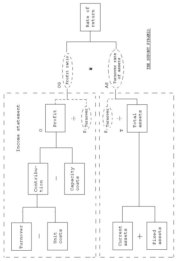
Figure 13.1

The Dupont Pyramid

.

- 68 -

13.2.1. Ratio mathematics, general

For the ratio U given by equation (282):

y

U = ¾¾¾ (282)

x

where y and x are system variable and/or system state functions, finan- cial or physical, the general function given by equation (283) applies in the same system:

y x₁ x_n x_n+1

U = ¾¾¾ ( ¾¾¾ - - - - ¾¾¾ ) ¾¾¾ (283)

x₁ x₂ x_n+1 x

In equation (283) x_i for i = 1, - - - -, n is an arbitrary quantity of system variable and/or system state functions.

If we define the ratio G₁ = y/x₁, G_i = x_i/x_i+1 for i = 1, - - - , n and G_n = x_n+1/x, equation (283) may be given the equivalent form:

U = G₁ G₂ G₃ - - - - G_n (284)

This is exactly the ratio technique forming the basis of the computati- on of the rate of return by the methods described in Section 13.2. (By the inserted variable S in equation (280) or by the product method in equation (281)).

A look at Bela Gold's work on managerial ratios will show that equati- ons (282), (283) and (284) constitute the theoretical contents of Bela Gold's application of ratios. It will be seen

.

- 69 -

that exactly the assumptions underlying equation (283) are the reason why the equation is not unique for a given system as regards the effect of the individual ratios on U. Thus, these effects can only provide cer- tain indications as to states in the system under study.

As a result of the above comments on the lack of uniqueness of a number of factors in a given development of a ratio, S, OG and AS are encircled by a broken line in Fig. 13.1.

The above equations provide the theoretical background of the uncertain- ty found in the literature on depiction of the Dupont pyramid. Thus, this pyramid is often shown without the S, OG and AS areas encircled by broken lines. The Dupont pyramid has a very simple memo-technical struc- ture. This structure consists of

The Dupont pyramid is a kind of rough aid for analysis purposes rather than a basic scientific figure with fundamental contents, cf. above.

.

- 70 -

Conclusion

The literature on the whole area of management, accountancy, manageri-

al economics and ratios has been reviewed. Only one source, lit. 30,

has been found suitable for a more detailed analysis in relation to

the management subject discussed: Managerial ratios.

As shown in Chapter A, S. Eilon's work takes as its starting point the

rate of return and defines a set of equations which under different

circumstances describe the effect of the rate of return. The assumpti-

ons underlying S. Eilon's equations are considered more closely, and

two weaknesses are found in the application of these equations. Eilon

uses the concept average variable costs, which is a generally applied

concept in tradi tional managerial economics. Eilon uses also an empi- rically based equation for the relationships between the sales activity and the funds tied up in the operating system. These two assumptions have given rise to the need for a continued theoretical development of the described mathematical functions as well as graphical models.

In Chapter B a graphical analytical business model is developed for

the purpose of giving management a picture of fundamental characteri-

stics in the business within bookkeeping, accountancy, managerial eco-

nomics and taxation. In Chapter B the mathematical functional expres-

sion for inventory depreciation is developed, equation (149), to form

the basis of the presentation of the relationship between O'_DS, B'_ln and O' in Fig. 2.1.

On the basis of the general graphical model with related mathematical

functions the mathematical analytical model is developed in Chapter C.

This model includes a number of definitions of general mathematical

functions as well as related parameters so that the developed functio- nal expressions give an analytical mathematical description of general-

.

- 71 -

concepts relating to book keeping, accountancy, managerial economics and taxation in the business on the basis of common input parameters, inclu- ding time as an explicit parameter.

Among the new functional expressions developed in Chapter C special

attention is called to the definition equation (174) together with the

condition equation (259) both of which form the basis of the develop-

ment of the general expression for cash flow released, see equation

(270). For assessments of the soundness of cash flow released, two ra-

tios have been developed, interest relative and depreciation relative,

see equati6n (271) and equation (272).

On the basis of the developed mathematical functions the traditional

ratios are presented in an analytical mathematical form as a function

of, among other things, time. To facilitate analysis, the complex func- tional expressions found have not been included in Chapter C, Section 13.

The Dupont pyramid, which forms the basis of the so-called "rate-of-

return philosophy", is in Fig. 13.1. divided into its basic components: Income Statement and Assets. The elements encircled by broken lines in Fig. 13.1., which are often omitted in representations, include the profit ratio and the turnover rate of assets. The development of the general ratio formula given by equation (283) has proved that the profit ratio and the turnover rate of assets are arbitrary accounting ratios.

With equation (283) and equation (284) the mathematical basis of the

computation of the rate of return and of Bela Gold's empirically deve-

loped ratio technique, lit. 40, has been developed.

.

- 72 -

BIBLIOGRAPHY

1. Ahlmark, Dan:

Produkt - investering - finansiering

Stockholm 1974

2. Andersen, A. Geel:

Investeringsteori. Partiel investeringsplanlægning under

sikkerhed

Copenhagen, The School of Economics and Business

Administration 1973

3. Ansoff, H. Iqor:

Strategisk planlægning

Copenhagen 1972

4. Arvidson, Herbert:

Foeretagsvaerdering, 3.

Stockholm 1978

5. Arwidz, Olof & Allan T. Maim:

Planeringssystem - en ram foer analys och konstruktion

Lund 1973

6. Asztely Sandor:

Investeringsplanering

Stockholm 1973

7. Bacharach, Michael:

Economics and the theory of games

London 1976

8. Baglini, Norman A:

Risk management in international corporations

New York 1971

9. Baker, A.J.:

Investment, valuation and the managerial theory of firm

Famborough 1978

10. Bannoch, Graham:

Smaller business in Britain and Germany

London 1976

11. Bergienut, P. och M. Hentzel:

Investering

Stockholm 1976

.

- 73 -

12. Bjarke, Ø. and 0.1. Franksen:

System structures in engineering. Economic design and

production

Lyngby The Technical University of Denmark, AMT 1978

13. Børsen PP3:

Erhvervenes og det offentliges udviklingsmønster fren til

1982.

Copenhagen 1977

14. Coates, C. Robert:

Investment strategy

London 1978

15. Coyle, R.G.:

Management system dynamics

London 1977

16. Cleland, David I. & William R. King:

Management. A system approach

New York 1972

17. Correa, Hector:

Integrated economic accounting Lexington,

Mass. 1977

18. Danielsson, Albert:

Foeretagsekonomi. Begreppsbildning och terminologie

Stockholm 1976

19. Danielsson, Albert:

Foeretagsekonomi - en oeversikt

Lund 1975

20. Danielsson, Albert:

On measurement and analysis of standard costs

Stockholm 1963

21. Dansk Management Center:

Inflationsregnskaber

Copenhagen 1978

22. Danø, Sven:

Introduktion til levetidsproblemer i investeringplanlægningen

Copenhagen 1978

23. Dam-Jensen, Erik m.fl.

Regnskab og økonomi

Copenhagen 1977

.

- 74 -

24. Donaldson, Gordon:

Strategy for financial mobility

Boston 1969

25. Donaldson, Peter & Jim Clifford:

Economy and decision making

London 1977

26. Dullum, K:

Virksomhedens økonomiske styring 1 & 2

Copenhagen 1975

27. Eckholm, Bo-Goeran:

Planering foer finansiell handlingsberedskap

Helsingfors 1977

28. EDB-rådet:

EDB, ledelse og økonomi

Copenhagen 1977

29. Eilon S. and Phocas-Cosmetatos G:

Analysis of profitability components. Proc. Euro II, Second

European Congress on Operations Research pp

143-147 ...... 1976

30. Eilon, Samuel & Cosmetatos, G.P.:

A profitability model for tactical planning

OMEGA, Vol. 5, No. 6 1977

31. Eilon, S., Gold Bela, and Soesan J.:

Applied productivity analysis for industry Pergamon Press,

Oxford 1976

32. Eliasson, Gunnar:

Business economic planning

Stockholm 1976

33. Fabryky, W.J. and G.J. Thuesen:

Economic decision analysis

Copenhagen 1974

34. Falster, P.:

Graph-oriented production models in APL Lyngby,

The Technical University of Denmark, 1977

35. Fiehn, Peter:

Produktionsstyring

Lyngby, The Technical University of Denmark, AMT 1978

.

- 75 -

36. Fog,Bjarke:

Mikroøkonomi

Copenhagen 1977

37. Forrester, Jay W.:

Industrial Dynamics

Cambridge, Mass. 1977

38. Gitman, Lawrence J.:

Principles of managerial finance

New York l976

39. Gold, Bela:

Explorations in managerial economics

London 1971

40. Gold, Bela:

Technological change. Economics, management and environment

Oxford 1975

41. Grant, Alexander Thomas Kingdom:

Economic uncertainty and financial structure

42. Greene, Mark R.:

Decision analysis for risk management

New York 1977

43. Grubbstroem, Robert W.:

Besluts- och spelteori med tillaempninger

Lund 1977

44. Gunst, Jens & Niels Lauritsen;

Planlaegning og prioritering

Copenhagen 1977

45. Hailes, William D. & Raymond T. Hubbard:

Small business management New York 1977

46. Hansen, Erik m.fl.:

Langtidsstyring

Copenhagen 1974

47. Hartley, W.C.F.:

Likviditetsstyringens ABZ

Institut for lederskab og 1ønsomhed

Copenhagen 1978

48. Hemming, Torn;

Multiobjective decision making under certainty

Stockholm 1978

.

- 76 -

49. Industrirådet:

Industriens Økonomi

Copenhagen 1977

50. Industriens Utredningsinstitut;

IUI's långtidsbedoemning 1976

Stockholm 1977

51. Jacobsen, Vagn Thorsgaard:

Valg af strategi og beslutning under usikkerhed

Copenhagen 1971

52. Jensen, A.:

Planlægning i uvished

Lyngby, The Technical University of Denmark,

IMSOR 1977

53. Jørgensen, Kj. Arnth:

Strategisk ledelse i mellemstore virksomheder

Danmarks Erhvervsfond 1977

54. Jørgensen, Niels Lihn:

Dynamisk input - output teori

Copenhagen 1977

55. Kallio, Markku:

Corporate planning model

Helsinki 1977

56. Keeney, Ralph L. & Howard Raiffa:

Decisions with multiple objectives

New York 1976

57. Keloharjn, Raimo:

Corporate modelling in system dynamics

Helsinki 1977

58. Kenessey, Zoltan:

Process of economic planning

New York 1978

59. Kline,John B.:

Management audit for small manufacturers

Wash. D.C. 1977

60. Kohn, Mervin:

Dynamic managing. Principles, process, practice

California 1977

.

- 77 -

61. Levy, Ham & Marshall Sarnst:

Capital investment and financial decisions

Englewood Cliffs. N.J. 1978

62. Lichtenberg, S.:

Projektplanlægning

Lyngby, The Technical University of Denmark 1978

63. Lin, Steven:

Conference on externalities, 1974. Southern Illinois

University. Theory and measurement of economic externalities.

New York 1976

64. Liung, Birger:

Investeringsbedoeinning

Stockholm 1978

65. Linestone, Harold A. & Devendra Sahal:

Technological substitution: Forecasting techniques and

applications

New York 1976

66. Longenecher, Justin G.:

Essentials of management

Illinois 1977

67. Lorange, Peter and others:

Strategic planning systems

Englewood Cliffs. N.J. 1977

68. MacKinzie, R. Alec..

New time management methods for you and your staff

London 1975

69. Martel, Jean Marc:

Adaptive strategies for a replacement problem

Louvain Univ. 1975

70. McLean, Ephraim R. & John V. Soden:

Strategic planning for MIS

New York 1977

71. Monks, Joseph G.:

Operations management. Theory and problems

New York 1977

72. Muhlemann, A.P. m.fl.

On portfolio modelling in multiple criteria situations

under uncertainty

Manchester 1977

.

- 78 -

73. Mulvaney,J.E. & C.W. Mann:

Practical business models

London 1978

74. Neergaard, Peter:

På basis af - - - - -

Thesis for the licentiate, The Copenhagen School of

Economics and Business Administration 1977

75. O'Connor, Rochelle:

Planning under uncertainty

New York 1978

76. Olsen, M. Kolbe:

Salgets planlægning og organisation

Copenhagen 1977

77. Papps, Ivy & Willie Henderson:

Models and economic theory

London 1977

78. Parker, J.E.S.:

Economics of innovation

London 1978

79. Petersen, Anders:

Konstruktion af systemer for økonomisk styrinq

Jern- og Metalindustriens Sammenslutning

Copenhagen 1976

80. Petersen, Eskild:

Målsætning i virksomheden

Copenhagen 1977

81. Peterson, Rein & Edward, A. Silver:

Decision Systems for inventory management and production

planning

New York 1978

82. Pfeffer, Irving:

Insurance and economic theory Illinois 1956

83. Pitchford, John D. & Stephen, J. Turnovsky:

Applications of control theory to economic analysis

Amsterdam 1977

84. Ramstroem, Dick:

Docentur I foeretagsekonomi

Uppsala 1977

.

- 79 -

85. Riis, Jens Ove:

Design of management Systems

Copenhagen 1978

86. Rasmussen,Flemming:

Eksempler på partiel investeringsplanlaegning

Copenhagen 1977

87. Rasmussen, Flemming:

Partiel investeringsplanlaegning

Lyngby, The Technical university of Denmark, IMSOR 1978

88. Rasmussen, G.:

Produktionsfunktioners anvendelse pA virksomhedsniveau

Lyngby, The Technical university of Denmark, AMT .....

89. Sandberg, Åke m.fl.:

Ny foeretagsekonomi

Stockholm 1978

90. Samuels, J.M. and Wilkes, F.M.:

Management of company finance

London 1975

91. Simon, Herbert A.:

New science of management decision

Englewood Cliffs., N.J. 1977

92. Siegwart, Hans:

Produktentwicklung in der industriellen Unternehmunq

Bern 1974

93. Sofka, Michael:

Marketingstrategie fuer ein neues Produkt

Diessenhofen 1971

94. Stemp, Isay:

Corporate growth strategies

New York 1970

95. Steuch, Axel:

Finansiel planlægning

Copenhagen 1977

96. Stone, Merlin:

Product planning

New York 1976

.

- 80 -

97. Sørensen, Finn C.:

Artikier om kreditvurdering og regnskabsanalyse

Copenhagen 1978

98. Siegel, Paul:

Strategic planning of management information systems

New York 1975

99. Steers, Richard M.:

Organizational effectiveness

California 1977

100. Struntz, Harald:

Langfristige Personalplanung auf der Grundlage von

Investitionsmodellen

Wiesbaden 1976

101. Sveriges Mekanfoerbund:

Nyckeltal i produktionen

Stockholm 1978

102. Sveriges Mekanfoerbund:

Produktivitetsmaetning

Stockholm 1978

103. Tamari, M.:

Financial ratios

London 1978

104. Thage, Bent & Jørn Holdt:

Input - output prismodel for Danmark

Copenhagen 1976

105. Twiss, Brian C.:

Managing technological innovation

London 1976

106. Wagner, Harvey M.:

Principles of operations research with applications to

managerial decisions

Prentice-Hall. Inc 1975

107. White, D.J.:

Fundamentals of decision theory

New York 1976

108. Williams, C. Arthur & Richards M. Hems:

Risk management and insurance

New York 1976

.

- 81 -

109. Wong, Kenneth Kin:

Risk analysis and control. A guide for DP managers

Manchester 1977

110. Worre, Zakken:

Vejledning i driftsbudgettering i den mindre virksomhed

Copenhagen 1974

111. Worre, Zakken:

Vejledning i likviditetsbudgettering i den

mindre virksomhed I og II

Copenhagen 1973

112. Young, Jerrald F.:

Decision making for small business in management

New York 1977