|
M
A S I The response of a linear sales
curve imposed to a micro
economical model of a company Hans Jessen Management Simulator M A S I , P.O. Box 171, DK-2630 Taastrup and Department of Mathematical Modelling The Technical
University of Denmark, DK-2800 Lyngby,
Denmark (November 11, 1998) Abstract A model of a company based on common accounting
practice for tactical planning is developed containing physical flow of materials,
manhours and deposits of materials, value flow and deposits of value and
financial flow and deposits as functions of time. In the first place a
graphical model is described naming each part by a mathematical function.
Thereafter the functions of time are determined with respect to accountancy
and their solutions are found imposing a linear sales curve. These solutions
describe fundamental functions in time of basic theory of accountancy with
reference to the flow of resources. E.g. profit and loss account, cash flow,
working capital and main key figures of the Dupont Pyramide are determined as
functions of time. Key words:
Flow of resources, accountancy, cash flow, working
capital, key figures, Dupont Pyramide. 1. INTRODUCTION This
paper is concerned with a model of a company containing common accoun- ting
practice. Such models have been presented by Bela Gold,7 with a keynumber technique, which were based on a
very simple ratio technique. Jay W. Forre- ster,6 developed models based on signal-graph - 2 - techniques,
but these models of system dynamics are difficult to apply in practice
because of the data to be found and to be interpreted. Models more applicable
for management analysis and decisions were developed by Albert Danielsson,2-3 in the form of flow-graphs but containing no
mathematical func- tions for evaluation. Samuel Eilon,4-5 made some mathematical approach to describe the
primary problem of this article, the equations as functions of time between
the working capital and the working system of profit and loss account,
without also considering the derived cash flow. His model as well as others
on this very aggregated data level are not able simultaneously to measure
values from the basic theory of accountancy as functions of time. In the litterature of accountancy
and management e.g. C. J. Malmborg,8
Alfred Rappaport,9 and R.S.
Segal,10 one will find no functions of time describing and
being consistent with accounting practice. Among
all these efforts to describe the processes of products and finance in a
company one will find Dan Ahlmark,1 as a primary source for this study. Dan Ahlmark only
made a general desciption without mathematical modelling of ac- countancy
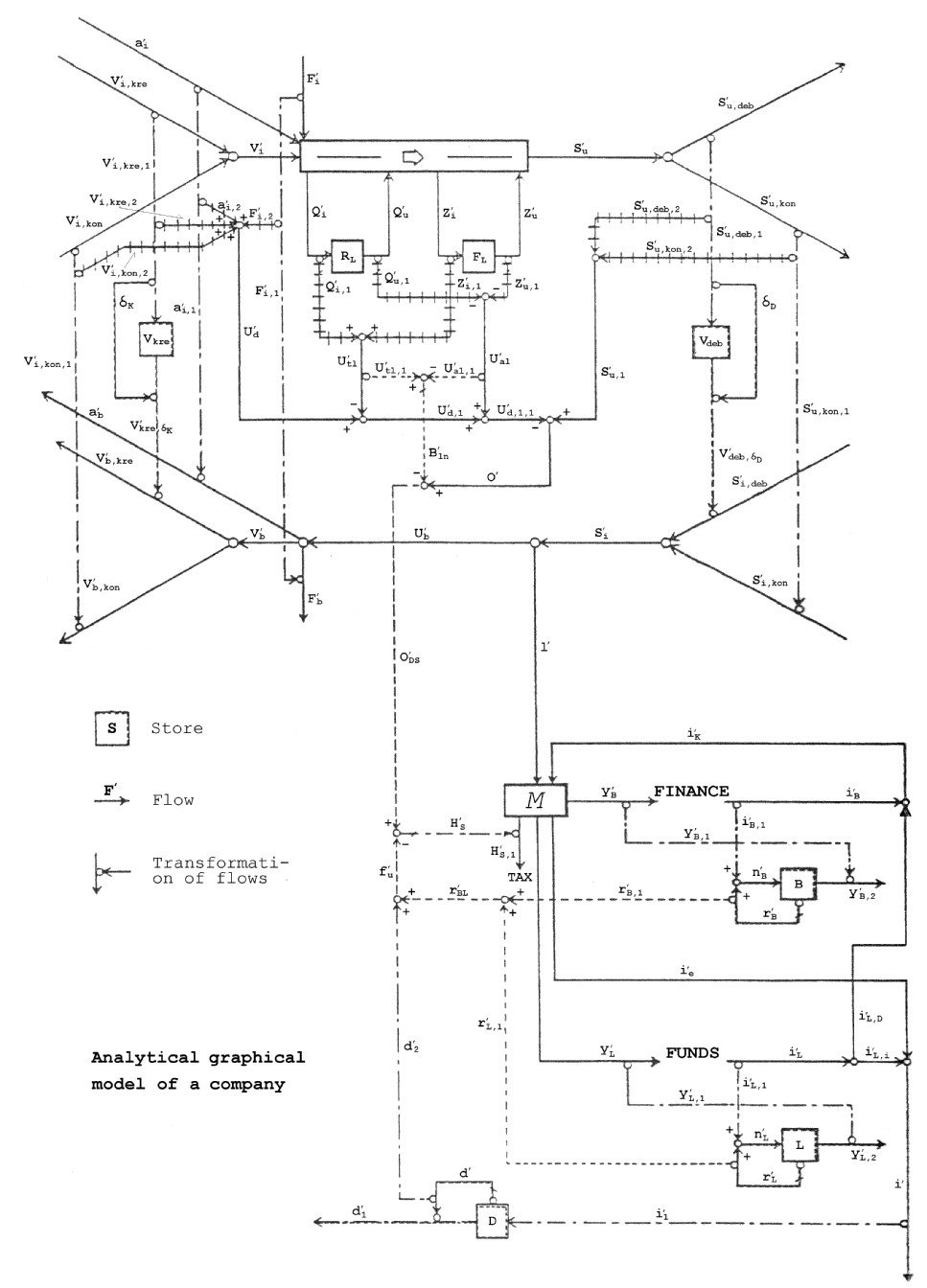
with functions of time. - 3 – 2. An
analytical graphical business model This
Chapter describes an analytical graphical business model (see Fig. 2.1.).
This model will form the basis of a mathematical analytical descrip- tion of
the business which can be used by the business management in their principal
planning activities. The model will integrate principal elements of
managerial economics and the accounting theory, under the assumption that the
business comprises an activity/ cash flow and related principal assets
(accounts payable, accounts receivable, inventories). It is the management's
task to achieve the best possible composition of this general structure by
using some of the ratios defined in the model. 2.1. Activity parameters 2.1.1. Sales The volume of goods sold by the firm per unit time
is denoted S'u, where S'u = S'u(t). The dot denotes the physial dimension of
“current”. Sales
are here divided into two main components of which one is the reference sales
S'u,kon, which refers to the share of
sales which is paid for in cash. The other component of sales is denoted with
S'u,deb, which refers to the share of sales
which is paid for by the trade accounts receivable the debit time dD after delivery from the firm. Here the following
eguation applies: S'u(t) = S'u,deb(t) + S'u,kon(t) (1) 2.1.2. Purchases The
firm is supplied with a number of labor hours per time unit denoted by a'i and with the volume of goods per time unit denoted
by V'i. The flow of goods consists of two main components
of which one is the reference purchase V'i,kon, and the other one in the goods purchased on credit
V'i,kre, which are
paid for by the firm after the credit time dK. - 4 –
- 5 - The
following equation applies: V'i(t) = V'i,kre(t) + V'i,kon(t) (2) The firm is supplied with the fixed volume of
resources per unit time F'i. This flow of resources may, for example, include
electricity, administration, heating, rent, etc. 2.1.3. Inventories The
volume Q'i of raw materials supplied per unit time is added to the raw materials inventory consisting
of the volume RL. From the
raw materials in- ventory is deduced the raw materials volume Q'u. The following equation appli- es here: t RL = ò (Q'i(t) - Q'u(t))dt (3) 0 The volume of finished goods per unit time Z'i is added to the finished goods inventory consisting of the volume FL. From the finished goods invento- ry is deduced the
finished goods volume Z'u. The following equation applies here: t FL = ò (Z'i(t) - Z'u(t))dt (4) 0 2.2. Payment parameters, operations 2.2.1. Sales The
total volume of means of payment per time unit from the customers is denoted
with S'i. This payments flow consists of two components. One
component is the payments flow S'i,kon caused by the cash sales flow S'u,kon. The other component S'i,deb is the payment flow caused by the credit sales flow
S'u,deb. Here the
following equation applies: S'i(t) = S'i,kon(t) + S'i,deb(t) (5) - 6 - 2.2.2. Purchases The
total volume of payment per unit time for operations is denoted by U'b. This payment flow is composed of three components,
a'b and V'b and F'b. a'b is the payment flow corresponding to the flow of
labour hours consumed a'i, V'b is the payment flow corresponding to the flow of
raw material purchases V'i, F'b is the payment flow corresponding to the flow of
fixed resources consumed F'i. The following equation applies: U'b(t) = a'b(t) + V'b(t) + F'b(t) (6) The
payments flow V'b is made up of two components. One component is the
pay- ments flow V'b,kon corresponding to the cash purchases of rawmaterials
V'i,kon; the other
component is the payments flow V'b,kre corresponding to the credit purchase of raw
materials V'i,kre. The following equation applies; V'b(t) = V'b,kon(t) + V'b,kre(t) (7) 2.3. Market parameters, sales In
order to depict the fundamental financial effects of the market on the firm
and its effects on earnings, the market is characterized by three basic
components q , p and dD. They also describe the fundamental link between
the firm's sales of goods and the related payment flows. 2.3.1. Cash sales ratio q The
cash sales ratio is defined by the equation: S'u,kon(t) = q S'u(t) (8) where
0 £ q £ 1
In
a manufacturing business q will typically have a value in the interval 0 £ q £ 0.2.
In a supermarket q will typically be in the interval 0.8 £ q £
1. - 7 - 2.3.2. The price p The
price of the firm's product(s) is defined by the eguations S'u,kon,1(t) = p S'u,kon(t) (9) S'i,kon(t) = S'u,kon,1(t) (10) where
S'u,kon,1(t) is the
flow of debts corresponding to the sales flow S'u,kon(t) (i.e. the current invoice flow stating the
amount of debt; see equation (9)). Equation (10) expresses the fact that the
flow of debts S'u,kon,1(t) is equal to the payments flow from the customers
(cash payment). In
practice, it should be noted that there is normally a time lag between
invoicing and sales. However, it has a temporary negative effect on liquidity
and the computation of results. Management will therefore have in view that
the invoicing is done without the mentioned delays. 2.3.3. Debit time dD This
model defines the debit time dD as the time of delivery of the goods from the firm
until the time of payment by the customer for the goods. In practi- ce, dD
is spread over the individual customers but with well defined terms of
payment the mean value can be detemined. The
definition of dD can be expressed by the equations S'u,deb,1(t) = p S'u,deb(t) (11) V'deb,dD(t) = S'u,deb,1(t - dD) (12) S'i,deb(t) = V'deb,dD(t) (13) - 8 - S'u,deb,1 refers here to the invoice flow corresponding to the
credit sales flow S'u,deb cf. equation (11). Equation (12) gives a functional
description of a function V'deb,dD(t), which can be defined as the payments flow (documents)
corresponding to the actual receipt of payments S'i,deb(t) cf. equation (13). In practice, no time lag is
found between the two last mentioned functions. In
pratice, attention should be paid to the fact that there may be a time lag in
the business between invoicing and sales, the result being changes in li-
quidity and the computation of earnings. Management usually aims at applying
equation (11) in practice, i.e. no time lag. 2.4. Market parameters, purchases With
a view to depicting the fundamental financial effects of the purchasing
market on the firm as well as its effects on costs, it is characterized by
four basic components e, q1,
q2 and dK. They describe the fundamental link between the
firm's purchases of resources and the related payment flows. 2.4.1. Cash purchases ratio e The
cash purchases ratio is defined by the equation: V'i,kon(t) = e V'i(t) (14) where
0 £ e £ 1 In,
say, a manufacturing business e will typically have a main value
in the interval 0 £ e £
0.2. This is also a typical
feature in a trading firm. 2.4.2. The price q1 of raw materials The
price of the firms raw materials is defined by the equation: - 9 - V'i,kon,1(t) = q1 V'i,kon(t) (15) V'b,kon(t) = V'i,kon,1(t) (16) where
V'i,kon,1(t) is the
flow of debts corresponding to the raw materials flow V'i,kon(t) (i.e. the current receipt of invoices stating
the amounts of debts); see equation (15). Equation (16) expresses the fact
that the flow of debts V'i,kon,1(t) is equal to the payments flow to suppliers (cash
payment). In
practice, attention should be paid to the fact that the time lag between the
supplier's invoicing and the supplies of raw materials is usually a temporary
feature which has a temporary positive effect on liquidity and the
computation of results. 2.4.3. The price q2 of labor hours The
price of the firm's labor hours is defined by the equations a'i,1(t) = q2 a'i(t) (17) a'b(t) = a'i,1(t) (18) where
a'i,1(t) is the
time ticket flow corresponding to the flow of labor hours used a'i(t) (i.e. the current issuing of time tickets
stating wages earned); see equation (17). Equation (18) expresses the fact
that the time ticket flow a'i,1(t) is equal to the time rate flow a'b(t). In
practice there is a certain time lag between functions on the right hand side
and the left hand side of the equal sign in equation (17). This time lag is
ignored here. There is usually no time lag between the functions of equa-
tion (18), or the time lag is relatively small and of no importance here. - 10 - 2.4.4. Credit time dK This
model defines the credit time dK as the time from the time of delivery of the raw
materials to the firm until the time of payment by the firm for the raw
materials. In practice, dK is spread over the individual suppliers but with
well defined terms of payment the mean value can be used. The definition of dK
can be expressed by the equations: V'i,kre,1(t) = q1 V'i,kre(t) (19) V'kre,dK(t) = V'i,kre,1(t - dK) (20) V'b,kre(t) = V'kre,dK(t) (21) where
V'i,kre,1(t) refers
here to the invoice flow corresponding to the credit purchases flow V'i,kre(t), cf. equation (19). Equation (20) gives a
functional description of a function V'kre,dK(t) which can be defined as the payment order flow
(documents) corresponding to the actual effecting of payments V'b,kre(t), cf. equation (21). In practice, there is no
time lag between the two last mentioned functions. In practice, attention should be
paid to the fact that the time lag between the supplier's invoicing and the
supplies of raw materials is usually a temporary feature which has a
temporary positive affect on liquidity and the computation of results. The
following equations are defined in relation to the fixed resources consumed F'i and the related fixed costs F'b. F'i,1(t) = k F'i(t) (22) F'b(t) = F'i,1(t) (23) - 11 - where
F'i,1(t) in
equation (22) refers to the flow of debts in the form of in- voices (stating
amounts) corresponding to the fixed resources flow F'i(t). k denotes a symbolic operator in the
form of an average price of the fixed re- sources unit. In practice, there is
some time lag between the functions in eguation (23). As, however, the fixed
costs by definition are constant in ti- me, such a time lag is not important
in this context. 3.1 Income statement In
this Chapter an income statement for operations is presented (before depre-
ciation, etc.) using the general main principles of accounting theory. 3.1.1 Sales of goods Sales
of goods are defined on the basis of the following equations: S'u,kon,2(t) = S'u,kon,1(t) (24) S'u,deb,2(t) = S'u,deb,1(t) (25) S'u,1(t) = S'u,kon,2(t) + S'u,deb,2(t) (26) Eguation
(24) expresses the fact that the flow of debts (in the form of in- voices
with statement of amounts) S'u,kon,1(t) gives rise to an equally large information flow
S'u,kon,2(t). This quantity
is identical with the current crediting to the cash sales account. From
equation (25) follows that the flow of debts S'u,deb,1(t) causes an equally large information flow S'u,deb,2(t). This quantity is identical to the current
crediting to the credit sales account. Total
sales in the form of the information flow S'u,1(t) corresponding to the total crediting to the
sales account are then obtained from equation (26). - 12 - 3.1.2 Costs The
costs of the firm in connection with production and sales are defined by the
following equations: V'i,kon,2(t) = V'i,kon,1(t) (27) V'i,kre,2(t) = V'i,kre,1(t) (28) a'i,2(t) = a'i,1(t) (29) F'i,2(t) = F'i,1(t) (30) U'd(t) = V'i,kon,2(t) + V'i,kre,2(t) + a'i,2(t) + F'i,2(t)
(31) Equation
(27) expresses the fact that the invoice flow from the cash purchase V'i,kon,1(t) is currently debited to the cash purchases
account to the extent of the cash flow V'i,kon,2(t). Equation
(28) expresses the fact that the invoice flow from the credit pur- chase V'i,kon,1(t) is currently debited to credit purchases account
to the extent of the cash flow V'i,kre,2(t). Equation
(29) denotes the functional relationship between the time ticket flow a'i,1(t) and the current debiting to the time rate
account of the wage payment flow a'i,2(t). Equation
(30) expresses the functional relationship between the invoice flow F'i,1(t) for fixed costs and the current debiting of the
cash flow F'i,2(t) to the fixed costs account. The
total cost flow is defined by equation (31). - 13 - 3.1.2.1 Inventories, additions (with signs)
By
way of introduction, it is mentioned that the signs relating to additions to
inventories (as a mean time value) are assumed to be the same as those
relating to additions to sales (as a mean time value). Against this
background the ad- ditions to the individual inventories will for principal
planning purposes ha-ve the same signs. The inventories only serve as
"standby stores" in case of emergency events "i.e. in normal
operation state" the materials and products go directly through the
factory. Thus, the following systems of equations apply: The
increase of sales S'u is supplied directly by the production and the
inventories are increased proportionally with S'u. Q'i(t) > 0 Q'u(t) = 0 d S'u ¾¾¾¾ >
0 Þ
(32) dt Z'i(t) > 0 Z'u(t) = 0 Constant
sales S'u is supplied directly by the production and the
inventories remain constant.
Q'i(t) = 0 Q'u(t) = 0 d S'u ¾¾¾¾ =
0 Þ
(33) dt Z'i(t) = 0 Z'u(t) = 0 The
decrease of sales S'u is supplied directly by the production and the flow
from inventories. The inventories are decreased proportionally with S'u. - 14 - Q'i(t) = 0 Q'u(t) > 0 d S'u ¾¾¾¾ < 0 Þ (34) dt Z'i(t) = 0 Z'u(t) > 0 The
system of equations (32) denotes that inventories rise when sales rise. The
system of equations (33) denotes that inventories are constant when sales
remain unchanqed. The
system of equations (34) denotes that inventories fall when sales fall. Based
on these main principles for the model the following equations can be
developed. Q'i,1(t) = qR Q'i(t) (35) Q'u,1(t) = qR Q'u(t) (36) Z'i,1(t) = qF Q'i(t) (37) Z'u,1(t) = qF Z'u(t) (38) U'tl(t) = Q'i,1(t) + Z'i,l(t) (39) U'al(t) = Q'u,1(t) + Z'u,1(t) (40) where Q'i,1(t) is the flow
of additions to raw materials invento-
ries corresponding to the additions to rawmateri-
als inventory records with statement of amounts. - 15 - Q'u,1(t) is the
flow of deductions to raw materials inven-
tories corresponding to the deductions to raw
materials inventory records with statement of
amounts. Z'i,1(t) is the
flow of additions to finished goods inven-
tories corresponding to the additions to finished
goods inventory records with statement of amounts. Z'u,1(t) is the
flow of deductions to finished goods inven-
tories corresponding to the
deductions to finished
goods inventory records with statement of amounts. qR denotes the calculated rav material price per
unit
of finished goods. qF denotes the calculated direct cost price per
unit
of finished goods. U'tl(t) is
total additions to inventories. U'al(t) is
total deductions from inventories. The
system of equations (32), (33) and (34) can now be given the form: d S'u ¾¾¾¾ > 0 Þ U'tl(t) > 0
and U'al(t) = 0
(41) dt d S'u ¾¾¾¾ = 0 Þ U'tl(t) = 0
and U'al(t) = 0
(42) dt d S'u ¾¾¾¾ < 0 Þ U'tl(t) = 0
and U'al(t) > 0
(43) dt Attention
is drawn to the fact that the physical model based on the FIFO principle can
be desribed mathematically only by - 16 - d S'u sign ( ¾¾¾¾ ) = sign (U'tl(t)) (44) d t given
U'al(t) = 0
(45) and
U'tl(t) is
computed with signs. 3.1.3. Resourceconsumption (incl. F'i,1) Resources
consumed U'd,1,1(t) can be defined by the following equations: d S'u ¾¾¾¾ > 0 Þ U'd,1,1(t) = U'd(t) - U'tl(t)
(46) dt given U'al(t) = 0 d S'u ¾¾¾¾ = 0 Þ U'd,1,1(t) = U'd(t) (47) dt d S'u ¾¾¾¾ < 0 Þ U'd,1,1(t) = U'd(t) + U'al(t)
(48) dt
given U'tl(t) = 0 3.1.4. Operation profit (before interest and
depreciation) The
operating profit (before interest and depreciation etc.) is defined by the
equation: O'(t) = S'u,1(t) - U'd,1,1(t) (49) 3.1.5 Operating profit incl. inventory
depreciation If a tax year of the length T is considered in a
period of time t1
£ t £ t1
+ T where t1 is a time
selected at random, the following functions can be defined: t1+T Vkøb = ò q1 V'i(t) dt (50) t1 w
= w(t1) (51) an = an(t) (52) - 17 - In
equation (50) Vkøb represents
the purchases of goods in the period
t1 £ t £ t1 + T. Equation
(51) defines w(t1) as the
total inventory value at time t1.
an(t) in the equation defines the inventory
depreciation rate. Materials
consumed computed for tax purposes is then derived from the follow- ing
equation (53): Vtax = Vkøb + w(t1) - (w(t1)/(1 - an(t1)) t1+T + ò (U'tl(t) - U'al(t)) dt) (1 - an(t1 + T)) (53) t1
For
principal planning purposes the mean time value of an(t)
for a given business will be a constant an and limited i.e. 0
< an < 0.3 . Based on this assumption equation (53)
gives
t1+T Vtax = Vkøb - (1 - an) ò (U'tl(t) - U'al(t)) dt (54) t1 Materials
consumed for operations is defined by the following equation:
t1+T Vdrift =
Vkøb + w(t1) - (w(t1) + ò (U'tl(t) - U'al(t)) dt)
(54a) t1 or t1+T Vdrift =
Vkøb - ò (U'tl(t) - U'al(t)) dt) (55) t1 If
equation (55) and equation (54) are combined, the following equations are
developed: t1+T Vtax = Vdrift + an ò (U'tl(t) - U'al(t)) dt (56)
t1 - 18 -
t1+T Vtax = Vdrift + ò an(U'tl(t) - U'al(t)) dt (57) t1
On
the basis of equation (57) the following functions can be defined: U'tl,1(t) = U'tl(t) (58) U'al,1(t) = U'al(t) (59) In
equation (58) U'tl,1(t) denotes total additions to inventories from a
taxation point of view. U'al,1(t) denotes in equation (59) total deductions from
invento-ries from a taxation point of view. With
the following definition equation: B'ln(t) = an (U'tl,1(t) - U'al,1(t)) (60) equation
(57) can be transformed into
t1+T Vtax = Vdrift + ò B'ln(t) dt (61) t1
On
the basis of equation (61) the following equation (62) can be defined: O'DS = O' - B'ln (62) where
O'DS is the
operating profit adjusted for inventory depreciation. 4.1. Change in liquidity (operations) The
cash flow released by operations, the change in liquidity, is defined by the
following equation (63): l'(t) = S'i(t) - U'b(t) (63) -
19 - 5.1. Cash balance The
cash balance of the firm is designated by M, which, in relation to the
present principal planning model, is very small in practice, i.e. M(t) = 0.
The folloving equation can now be developed: i'e = l' + i'K - y'B - y'L - H'S,1 (64) where
i'e is the
self financing flow y'B is the
service of bank loans y'L is the
service of other loans i'K is
current raise of loans for operations H'S,1 is tax
payments 5.2. Bank loans. The
firm is financed currently by trading credits in the form of the cash flow i'B. The equation is defined as follows: i'B,1(t) = i'B(t) (65) where
i'B,1(t) is the
information flow in the form of loan documents with statement of amounts
corresponding to the cash flow i'B(t). The bank charges currently interest r'B(t) on the amount outstanding B
= B(t) where r'B(t) is the document flow with statement of interest.
The following equation applies: n'B(t) = i'B,1 + r'B (66) where
n'B(t) is the
firm's current crediting to the bank account. - 20 - The
current service payments y'B(t) to the bank give rise to a payment order flow
with statement of amounts y'B,1(t). We have: y'B,1(t) = y'B(t) (67) The
payment order flow y'B,1(t) involves a corresponding current debiting to the
bank account in the form of y'B,2(t). The following equation therefore ap- plies: y'B,2(t) = y'B,1(t) (68) 5.3. Loans (long term) The
long term financing of the business is represented by the cash flow i'L. The following equation applies: i'L,1(t) = i'L(t) (69) where
i'L,1(t) is the
information flow in the form of loan documents with statement of amounts
corresponding to the cash flow i'L(t). On the loan L current interest r'L(t) is charged where r'L(t) is the document flow with statement of interest.
The following equation applies: n'L(t) = i'L,1(t) + r'L(t) (70) where
n'L(t) is the
firm's total current crediting to the loan account. The
following equation applies: i'L(t) = i'L,1(t) + i'D(t) (71) where
i'L,D(t) denotes
the long term financing flow to the working capital, and i'L,1(t) is the long term financing flow to the fixed
capital. - 21 - The
folloving equation applies: i'K(t) = i'B(t) + i'L,D(t) (72) The
current service payments y'L(t) to lender give rise to a payment order flow with
statement of amounts y'L,1(t). We have y'L,1(t) = y'B(t) (73) The
payment order flow y'L,1(t) involves a corresponding current debiting to the
loan account in the form of y'L,2(t). The following equation therefore applies: y'L,2(t) = y'L,1(t) (74) 6.1. Investment (in fixed capital) The
firm's current investment in fixed capital is denoted i'(t). The following equation applies: i'(t) = i'L,1(t) + i'e(t) (75) It
is pointed out that, in practice, i'L,D(t) currently converts short term liabilities into
long term liabilities, which means that at a strategic level alone i'L,D = 0. As to i'e(t), there is no unique definition of i'e(t) as it de- pends on the financing and market
situation. Roughly speaking, i'e(t) is the average cash flow which can be withdrawn
from the business without changing the existing product, investnent and
financing structure and the necessary financial reserves set aside for an
appropriate future development of the bu- sinees. - 22 - 7.1. Depreciation (for tax purposes) It
is normal to distinguish between depreciation for tax purposes and depre-
ciation for accounting purposes. Depreciation for accounting purposes is used
with the object of comparing alternative projects on the basis of special
cost principles. These principles are purely OR mathematical models and do
not reflect the physical business situation. Here
we shall only take an overall view of the financial flow of the firm for
which reason depreciation for tax purposes will be used. Such depreciation
will only reflect the actual effects on liquidity (after tax). The
following equations apply: i'1(t) = i'(t) (76) t D(t) = ò (i'1(t) - d'1(t))dt (77) 0 where
i'1(t)
represents the current debiting to the tax depreciation account corresponding
to the investment flow i'(t). d'1(t) is the current crediting to the same account
(i.e. current "depreciation"). D(t)
represents the balance of the tax depreciation account. The depreciation
charges d'(t)
are calculated on the basis of this account, and the following expressions
apply: d'1(t) = d'(t) (76a) d'2(t) = d'(t) (76b) where
d'2(t) is the
depreciation flow which is included on the basis of compu- tation of the
taxable income. - 23 - 8.1. Interest (for tax puroses) Interest
is usually computed for two main purposes. One concerns the income statement
for tax purposes, the other concerns internal computation purposes such as
the effect of interest on the income statement as a whole or in con- nection
with special computations. No
distinction will be made here between the two purposes. The interest charges
will be placed in this model with the sole aim of depicting the fundamental
fi-nancial characteristics. The
following equations are defined: r'B,1(t) = r'B(t) (78)
r'L,1(t) = r'L(t) (79) r'BL(t) = r'B,1(t) + r'L,1(t) (80) where r'B,1(t) denotes the current recording of interest
payment to the bank. r'L,1(t) denotes the current recording of interest
payments to other lenders. The recording of total interest payments is
designated r'BL(t). 9.1. Tax payments According
to the principles governing computation of the taxable income the following
equations apply: f'u(t) = d'2(t) + r'BL(t) (81) H'S(t) = s (O'DS(t) - f'u(t)) (82) H'S,1(t) = H'S(t) (82a) - 24 - where
f'u(t) is a
state function for the computation of tax, cf. equation (81), s is the
tax rate, H'S(t) is the computed tax payment and H'S,1(t) is the tax payment flow. 10.1. Principal ratios As
appears from Fig. 2.1, the following principal ratios in the firm are
im-portant to the understanding of the dynamic (tactical) characteristics of
the firm. Operating profit O'(t) Change in liquidity l'(t) Working capital (net) K'(t) Contribution ratio DG(t) Depreciation d'2(t) Interest r'BL(t) These
ratios will be discussed in detail in the following. 10.1.1. Operating profit O'(t)
Using
different assumptions concerning prices and changes in principal assets
(accounts payable, accounts receivable, inventories) it is possible via Fig.
2.1 to assess the effects on the operating profit. A reduction of the raw
materials inventories in a situation with raw materials prices which are
higher than the prices of the raw materials inventories but otherwise
constant will increase the profit temporarily in the period concerned. One
of the things that will be seen is that the profit O'(t) is independent of the volume of trade accounts
payable and the volume of trade accounts recei- vable. - 25 - 10.1.2. Change in liquidity l'(t)
Other
things being equal, the following expression, cf. Fig. 2.1., applies: d S'u ¾¾¾¾ > 0 Þ l'(t) < O'(t) (83) d t Equation
(83) shows that the profit O'(t) is larger than the change in liqui- dity in the
case of growing sales in the firm, the reason being the funds ti- ed up,
calculated with signs, in principal assets (accounts receivable and
inventories), d S'u ¾¾¾¾ = 0 Þ l'(t) = O'(t) (84) d t Equation
(84) shows that the change in liquidity is equal to the profit in the case of
constant sales, the reason being an unchanged volume of principal as-sets
(accounts payable, accounts receivable and inventories). d S'u ¾¾¾¾ < 0 Þ l'(t) > O'(t)
(85) d t From
equation (85) appears that in the case of falling sales the change in
liquidity becomes greater than the operating profit owing to a reduced volume
of principal assets (accounts payable, accounts receivable and inventories). The
above shows how important it is for the business to keep the cash budget
currently up to date as the profit and the financial circumstances of the
business may differ substantially from each other. It should be noted that if
the net principal assets are negative, the inequality signs in (83) and (85)
must be reversed. - 26 - 10.1.3. Working capital K(t) If
the working capital is denoted K(t), the definition eguation for net capi-
tal tied up in the operating system will apply: K(t)
= Vdeb(t) + FL(t) + RL(t) - Vkre(t) (86) The
following definition equation will also apply: d K(t) ¾¾¾¾ + l'(t) = O'(t) (87) d t Equation
(87) shows that the profit is equal to the change in liquidity + the
increment of the net working capital tied up. If
equation (87) is transformed, the following equation is derived: d K(t) ¾¾¾¾ = O'(t) - l'(t) (88) d t Equation
(88) denotes that the difference between the operating profit and the change
in liquidity is equal to the financing requirements for operations in the
period under review. 10.1.4. Contribution ratio DG(t) The
contribution ratio is defined by equation (89): DG(t)
= (O'(t) + F'b(t))/S'u,1(t) (89) Equation
(89) shows that DG is independent of the amount of sales and defines the
share of sales which will cover fixed costs, etc. The point is stressed here
that a high contribution ratio does not imply that there is "money"
to cover the fixed costs. For further details see section 10.1.2. as the size
of l'(t)
gives only an indication of the ability of the firm to pay fixed costs, etc. - 27 - 10.1.5. Depreciation Depreciation
contributes to influencing the firm's liquidity, cf. equation (82). Assuming
that the investments are made as individual projects at time intervals, it is
shown that depreciation in the periods between investments causes liquidity
to rise owing to the reduction in tax payments. However,
it should be noted that of the cash flow released after tax there must be
funds to cover repayment commitments in connection with loans raised. The
effect of the cash flow released after tax described above is therefore
partial and must be seen in relation to the repayment commitments. Later
there will be shown that for practical reasons the division described here is
desirable for the understanding of the financial components of the cash flow
released. 10.1.6. Interest r'BL From
Fig. 2.1 and from equations (81) and (82) is apparent that interest pay-ments
reduce the cash flow released after tax. Thus, the net effect on cash flow released (to be defined
later) stems partly from the computation of income for tax purposes, partly
from the payment of interest on total loans. The
computation of interest on total loans seen in relation to a given level of activity
will be defined later. - 28 - 11. An analytical mathematical business
model This
Chapter presents a new analytical mathematical model description of the
business. This model has been developed for use in the tactical planning pro-
cess. No reference can be made to a similar model in existing literature. The
theoretical literature which gets nearest is S. Eilon's article discussed in
Chapter A in “Economical Keynumbers”. 11.1. Physical and financial functions in the
operating system In
the following further definitions of mathematical functions and their rela-
tionships will be established. The sole justification of these definitions is
that they provide the basis of a clear and generally coherent system of
equa-tions between ratios. 11.1.1. Sales A
basic sales volume is defined: S'u0 = S'u(0) (90) where
S'u0 is the
volume of sales S'u at time t = 0, i.e. at the beginning of the
simulation period. The
development of sales during the time period is defined by equation (91): d S'u(t) ¾¾¾¾
= as S'u0 (91) d t where
as is constant. - 29 - The
following equation now applies: S'u(t) = S'u0(1 + as t) (92) where
t ³ 0 11.1.2. Inventories Let
a ratio hF be defined
so that equation (93) applies: hF = FL(t)/S'u(t)
(93) for
t ³ 0, hF being a positive constant which is designated
"finished goods inventory time". Another ratio hR is defined so that equation (94) applies: hR = RL(t)/S'u(t) (94) for
t ³ 0 being a
positive constant which is designated "raw materials inventory
time". From
equation (93) follows: FL(t) = hF S'u(t) (95) The
definition equation applies: t FL(t) = FF(0) + ò Z'i(t) dt (96)
0 which
substituted into equation (95) gives: |
|
- 30 - t FL(0) + ò Z'i(t) dt = hF S'u(t) (97) 0 or
t ò Z'i(t) dt = hF S'u(t) - FL(0) (98) 0 If
equation (92) is used in equation (98), the following expression is derived: t ò Z'i(t) dt = hF S'u0 as t + (hF S'u0 - FL(0)) (99) 0 For
t = 0 equation (93) gives the following expression: hF = FL(0)/S'u(0) (100) Using
equation (100) together with equation (99) we have: t ò Z'i(t) dt = hF S'u0 as t (101) 0 The
solution to the integral equation (101) is: Z'i(t) = hF S'u0 as
(102) The
flow of goods Z'i(t) to the finished goods inventory may then be
defined by equations (103) and (104): Z'i(t) = hF S'u0 as
(103) for
as ³ 0 and
- 31 - Z'u(t) = - hF S'u0 as
(104) for
as < 0 Mathematically
the physical equations (103) and (104) may be described by equation (105) for
all values of as, i.e. Z'i(t) = hF S'u0 as
(105) for - ¥ < as < ¥ With
equation (105) the physical inventory system has been converted to a
mathematical model where Z'i(t) can change sign and where Z'u(t) = 0 for all t, cf. equation (102). From
equation (94) follows: RL(t) = hR S'u(t) (106) The
definition equation applies:
t RL(t) = RL(0) + ò Q'i(t) dt (107)
0 which
combined with equation (106) gives: t RL(0) + ò Q'i(t) dt = hR S'u(t) (108) 0 or
t ò Q'i(t) dt = hR S'u(t) - RL(0) (109) 0 If
equation (92) is used in equation (109), the following equation is derived: - 32 - t ò Q'i(t) dt = hR S'u0 as t + (hR S'u0 - RL(0)) (110) 0
For
t = 0 equation (94) gives: hR = RL(0)/S'u(0) (111) Using
equation (110) together with equation (111) we have: t ò Q'i(t) dt = hR S'u0 as t
(112) 0 The
solution to the integral equation (112) is: Q'i(t) = hR S'u0 as
(113) The
flow of goods Q'i(t) to the raw materials inventory can now be
defined by equations (114) and (115): Q'i(t) = hR S'u0 as
(114) for
as ³ 0 Q'u(t) = - hR S'u0 as (115) for
as < 0 Mathematically
the physically equations (114) and (115) can be described by equation (116)
for all values of as,
i.e. Q'i(t) = hR S'u0 as
(116) for - ¥ < as < ¥ With
equation (116) the physical inventory system has been converted to a
ma-thematica1 model where Q'i(t) can change sign and where Q'u(t) = 0 for all t. - 33 - 11.1.3. Output Total
output T'p(t) is given by: T'p(t) = S'u(t) + Z'i(t) (117) If
the ratio ba is here
defined as the number of labor hours used per unit of output and the ratio bR as the raw materials consumption per unit of
finished goods, the equations, resource balance equations, will apply: a'i(t) = ba T'p(t) (118) V'i(t) = bR T'p(t) + Q'i(t) bR (119)
If
equation (117) and equation (119) are combined, the following equation is
obtained: V'i(t) = bR S'u(t) + bR Z'i(t) + Q'i(t) bR (120) If
equations (92), (105) and (116) are substituted into equation (120), the
following equation is obtained: V'i(t) = bR S'u0 (1 + (hF + hR + t) as) (121) Using
equations (117), (92) and (105), equation (118) gives: a'i(t) = ba S'u0 (1 + as(t + hF)) (121a) 11.1.4. Sales, ingoing payments Using
equations (8), (9) and (10) we obtain payments derived from cash sales: S'i,kon(t) = p q S'u0 (1 + as t) (122) - 34 - Using
equations (1), (8), (11), (12) and (13) we obtain payments derived from debit
sales: S'i,deb(t) = p (1 - q) S'u0 (1 + as(t - dD)) (123) Equations
(1), (122) and (123) give: S'i(t) = p q S'u0 (1 + as t) + p (1 - q) S'u0 (1 + as(t
- dD)) (124) or
S'i(t) = p S'u0 (1 + as(t - dD(1 - q))) (125) 11.1.5. Purchases, outgoing payments The
outgoing payments flow corresponding to cash purchases of raw materials is
expressed by means of equations (14), (15), (16) and (121) as V'b,kon(t) = q1 e bR S'u0 (1 + (hF + hR + t)as) (126) Credit
purchases of raw materials cause an outgoing payments flow which by means of
equations (7) (14), (19), (20) and (21) is computed at: V'b(t) = e q1 V'i(t) + (1 - e)q1 V'i (t - dK) (127) Equation
(127) is transformed by means of equation (121) into: V'b(t) = e q1 bR S'u0(1 + (hF + hR + t) as) + (1 - e)q1
bR S'u0(1 + (hF + hR
+ t - dK)as) (128) Equation
(128) is reduced to: V'b(t) = q1 bR S'u0(1 + as(hF + hR + t - dK (1 - e))) (129) - 35 - The
total payments flow to purchases of resources is then obtained by using
equations (6), (17), (18) and (129): U'b(t) = q2 a'i(t) + q1 bR S'u0(1 + as (hF + hR + t - dK (1 - e))) + F'b(t) (130) By
combining equation (121a) and equation (130) the total outgoing payments flow
is then given by: U'b(t) = S'u0(q2
ba (1 + as (t + hF))
+ q1 bR(1
+ as (hF + hR + t - dK(1 - e))) + F'b(t) (131) 11.1.6. Change in liquidity The
accounting concept, change in liquidity l'(t), here also called cash flow, can then by the use
of equations (63), (125) and (131) be given the following form: l'(t) = S'u0(p(1 + as(t - dD(1 - q))) - q2
ba (1 + as(t + hF))
- q1 bR(1
+ as
(hF + hR + t - dK(1 - e)))) - F'b(t)
(132) 11.2. Capital tied up in the operating system
Depending
on the firm's level of activity capital will be tied up in the ope- rating
system. Capital will be tied up in trade accounts payable, raw materi- als
inventories and finished goods inventories as well as accounts receivable
(the amounts are indicated with signs). 11.2.1. Trade accounts receivable The
volume of trade accounts receivable is defined by the following equation,
equations (1), (8), (11) and (12) being used: dD Vdeb(t) = ò p(1 - q)S'u(t - x) dx (133) 0 - 36 - In
this model it is assumed that equation (92) applies. From this equation
combined with (133) follows: dD Vdeb(t) = p(1 - q) S'u0 ò (1 - as(t - x)) dx (134)
0 The
computation of the integral in equation (134) allows equation (134) to be
reduced to: Vdeb(t) = p(1 - q) S'u0 dD (1 + as(t - 0.5 dD)) (135) 11.2.2. Trade accounts payable The
volume of trade accounts payable is defined by the following equation,
equations (2), (14), (19) and (20) being used: dK Vkre(t) = ò q1 bR(1 - e) V'i(t - x)) dx (136) 0 Assuming
that sales satisfy equation (92) and that equation (121) applies, equation
(136) develops the following expression: dK Vkre(t)
= q1 bR(1
- e) S'u0 ò (1 + as(hF + hR
+ t - x)) dx (137) 0 By
computing the integral in equation (137) this equation is reduced to: Vkre(t) = q1 bR(1
- e) S'u0 dK (1 + as(hF
+ hR + t - 0.5 dK))
(138) l1.2.3 Raw materials inventory The
volume of the raw materials inventory is given by equation (106). The value
of the raw materials inventory RL,1(t) satisfies the equation: RL,1(t) = q1 bR RL(t)
(139) - 37 - If
equations (106) and (92) are substituted into equation (139), we have: RL,1(t) = q1 bR hR S'u0(1 + as t) (140) 10.2.4. Finished goods inventory The
volume of the finished goods inventory is given by equation (95). The
calculated consumption of materials and labor hours per unit of finished
goods is given by qF,
cf. equation (37). The definition equation applies: qF = bR
q1 + ba
q2 (141) The
value of the finished goods inventory FL,1(t) satisfies the equa-ion: FL,1(t) = qF FL(t) (142) If
equations (95), (92) and (141) are substituted into equation (142), the
following expression is obtained: FL,1(t) = (bR q1 + ba q2) hF S'u0(1 + as t) (143) 11.2.5. Working capital (tied up in the
operating system) The
total capital tied up in the operating system, i.e. the working capital K(t),
is through the use of equations (135), (138), (140) and (143) given by: K(t)
= Vdeb(t) - Vkre(t) + RL,1(t) + FL,1(t) (144) or
by substituting into the relevant places K(t) = p(1 - q)S'u0 dD (1 + as(t - 0.5 dD)) - q1 bR (1 + e)S'u0 dK (1 + as(hF + hR + t - 0.5 dK)) + q1 bR hR S'u0(1 + as t) + (bR
q1 + ba
q2) hF
S'u0(1 + as t) or - 38 - K(t) = S'u0(1 + as
t)(hF (bR
q1 + ba
q2) + q1
bR hR)
+ p(1
- q) dD S'u0(1 + as(t
- 0.5 dD)) - q1 bR
(1 - e) dK S'u0(1 + as(hF + hR + t - 0.5 dK))
(145) 12.1. Operating profit (for accounting
purposes) In
the following, functions are established for the computation of operating
profit based on accounting theory. The
turnover of the firm is obtained by using equations (9), (11), (24), (25) and
(26) and is expressed as: S'u,1(t) = p S'u(t) (146) Using
equation (92) and equation (136) gives: S'u,1(t) = p S'u0(1 + as t) (147) Raw
materials consumed corresponding to sales S'u(t) are given by the equation: V'for(t) = q1 bR S'u(t) (148) or
by using equation (92): V'for(t) = q1 bR S'u0(1 + as t) (149) The
wages paid, time rates, corresponding to sales S'u(t) are given by the equation: a'for(t) = q2 ba S'u(t) (150) or by using equation (92) a'for(t) = q2 ba
S'u0(1 + as t) (151) - 39 - By
using equations (147), (149) and (151) the operating profit O'(t) can now be given the form: O'(t) = S'u,1(t) - V'for(t) - a'for(t) - F'b(t) (152) or
O'(t) = S'u0(1 + as
t)(p - (q1 bR + q2
ba)) - F'b
(153) 12.2. Operating profit (computed on the basis
of Fig. 2.1) In
this section the operation profit will as an alternative be computed directly
on the basis of Fig. 2.1. The
costs U'd(t) in connection with sales S'u(t) are given by equation (31). If equations (2),
(15), (17), (19), (22), (23), (27), (28), (29), (30), (121) and (121a) are
substituted into equation (31), the following equation is de veloped: U'd(t) = q1 bR
S'u0(1 + (hF + hR
+ t) as) + q2 ba
S'u0(1 + (hF + t)as)
+ F'b (154) Computed
with a plus or minus sign (positive for inventory) the following va- lue is
added to the raw materials inventory, cf. equation (35): Q'i,1(t) = q1 bR Q'i(t) (155) or
equation (116) may be used: Q'i,1(t) = q1 bR
hR S'u0 as
(156) Here
the definition equation for cost prices of raw materials per unit of finished
goods has been used: qR = q1
bR (157) - 40 - The
following value is added to the finished goods inventory, cf. equation (37): Z'i,1(t) = qF Z'i(t) (158) or
equation (102) may be used: Z'i,1(t) = (q1 bR
+ q2 ba)
hF S'u0 as (159) The
total value flow to inventories now amounts to, cf. equations (44) and (45): U'tl(t) = q1 bR
hR S'u0 as
+ (q1 bR
+ q2 ba)
hF S'u0 as (160) or
by reduction U'tl(t) = S'u0 as(q1 bR
hR + (q1 bR
+ q2 ba)
hF) (161) The
total operating profit is obtained by using equations (147), (154) and (161)
and is expressed as: O'(t) = S'u(t) - (U'd(t) - U'tl)) (162) or
by substituting into the right hand side: O'(t) = p S'u0(1 + as t) - (q1
bR S'u0(1 + (hF + hR
+ t) as) + q2 ba
S'u0(1 + (hF + t) as) + F'b - S'u0 as
(q1 bR
hR + (q1 bR
+ q2 ba)
hF))
(163) - 41 - or
by reduction: O'(t) = S'u0(1 + as t)(p -(q1 bR + q2 ba)) - F'b
(164) It
will be seen that equations (153) and (164) are identical, i.e. a systema- tic
use of Fig. 2.1. gives here the same result as the use of a simple
"logi- cal" accounting method. 12.2.1. Operating profit incl. inventory
depreciation If
equations (161) and (58) are substituted into equation (60), U'tl,1(t) being computed with a plus or minus sign, the
following equation is obtained: B'ln(t) = an S'u0 as (q1
bR hR
+ (q1 bR
+ q2 ba)
hF)
(165) The
operating profit incl. inventory depreciation is given by equation (62). If equations
(164) and (165) are substituted into this equation, the following expression
is derived: O'DS(t) = S'u0(1 + as
t)(p -(q1 bR + q2
ba)) - F'b -
an S'u0 as (q1
bR hR
+ (q1 bR
+ q2 ba)
hF)
(166) or by reduction: O'DS(t) = S'u0((1 + as t)(p -(q1 bR
+ q2 ba)) - an as (q1
bR hR
+ (q1 bR
+ q2 ba)
hF) - F'b (166a) - 42 - 12.3.1. Bank loans This
model takes as its starting point that the net working capital tied up K(t)
can be given the form: K(t)
= K0 + Kinc(t)
(167) where
K0 is the net working capital tied up at time t = 0,
and Kinc(t) is the
change in the working capital tied up at time t. It is assumed that equation
(168) applies: d Kinc(t) ¾¾¾¾¾ = i'B(t) (168) d t This
means that the increase in the capital tied up in the operating system is
financed by the bank overdraft. If
equation (168) is used together with equation (167), the following equation
will also apply: d K(t) ¾¾¾¾¾ = i'B(t) (168a) d t It
is assumed that: B(0)
= 0 (169) This
means that the overdraft amounts to DKK B(0) = 0 at time t = 0. As
regards the mathematical model it is pointed out that in equation (168) i'B(t) may be both positive and negative as it is also
assumed here that, besides equations such as (65), (66), (67) and (68), the
following equation applies: y'B(t) = r'B(t) (170) - 43 - 12.3.2. Loans (long term) It
is assumed that i'L(t) is discreet, i.e. that i'L(t) = 0 and i'D(t) = 0 (171) for
all t > 0, apart from certain selected times tq where, in
practice, chan-ges take place in financing conditions, and new investments
are made. Subject to these assumptions equation (72) may be reduced to i'K(t) = i'B(t) (172) with
the condition i'L,D(t) = 0 In
close connection with the operational financial possibilities of equations
(171) and (172) this model also assumes that equation (173) applies: y'L(t) = r'L(t) (173) 12.3.3. Investments Investments
are defined by i'(t). It is here assumed that i'(t) = 0 apart from certain times tp corresponding to the forms of investment seen in
practice. In
this mathematical model equation (75) is changed into: i'(t) = i'L,i(t) (174) where
i'e(t)
thereafter becomes the quantity, cash flow released, for the following
purposes: - 44 - New investments Instalments on
loans Etc. This
change of equation (75) is desirable seen in relation to the possibili- ties
of implementing this mathematical model on a computer. 12.4.1. Interest payments From
equations (78), (79), (80), (170) and (173) the total interest payment is
derived: y'B(t) + y'L(t) = rB B(t) + rL L(t) (175) where
rB is interest rate bank and rL is interest rate lender. 12.4.2.
Depreciation Depreciation
to tax computation is obtained from equation (77) and is expressed as: d'2(t) = aD D(t) (176) where aD is the depreciation rate per time period. 12.4.3. Tax payments From
equations (81), (175) and (176) the following equation is derived: f'u(t) = aD D(t) + rB B(t) + rL L(t) (177) By
using equations (82) and (177) total tax payments are expressed as: H'S,1(t) = s(O'DS(t) - aD D(t) - (rB B(t) + rL L(t)))
(178) - 45 - 12.4.4. Cashflow released With
the special definition of i'e(t) given in 12.3.3. cash flow released is defined
by: i'e(t) = O'(t) - H'S,1(t) - (y'B(t) + y'L(t)) which
together with equation (88) gives: i'e(t) = l'(t) + dK(t)/dt - H'S,1(t) - (y'B(t) + y'L(t)) If
equation (168a) including the related assumption is used here, the follow-
ing equation is obtained: i'e(t) = l'(t) - H'S,1(t) - (y'B(t) + y'L(t)) + i'B(t)
(179) or
if equations (175) and (178) are used: i'e(t) = l'(t) + i'B(t) - s O'DS(t) + s aD D(t) - (1 -
s)(rB B(t) + rL L(t)) (180) By
using equations (62) and (87), the following equation is derived from
equation (180): i'e(t) = O'(t) - s O'DS(t) + s aD D(t) - (1 -
s)(rB B(t) + rL L(t)) (181) If
the function O'L(t) is defined by the equation: O'L(t) = O'(t) - s O'DS(t) (182) O'L(t) may be designated as the profit after tax from the
operating system. Equation
(181) is now transformed into: i'e(t) = O'L(t)(1 + s aD D(t)/O'L(t) - (1 -
s)(rB B(t) + rL L(t))/O'L(t) (183) It
appears from equation (183) that it may be appropriate to define the fol-
lowing managerial ratios: - 46 - 12.4.4.1. Interest relative Interest
relative is defined by equation (183): rB B(t) + rL L(t) rrel = - (1 - s) ¾¾¾¾¾¾¾¾¾¾¾¾ (184)
O'L(t) rrel can be interpreted as interest payments after tax
in relation to profit after tax from the operating system. 11.4.4.2.
Depreciation relative Depreciation
relative is defined by equation (183): aD D(t) arel
= s ¾¾¾¾¾¾¾ (185)
O'L(t) arel may be interpreted as the improvement in cash flows
after tax as a result of depreciation in relation to profit after tax from
the operating system. - 47 - 13.1. Traditional ratios In
this Chapter some traditional ratios will be computed on the basis of the
functional expressions derived in section 12. 13.1.1. Contribution ratio The
contribution ratio DG(t) is defined by the following equation (186): S'u,1(t) - (U'd,1,1(t) - F'i,2(t)) DG(t) = ¾¾¾¾¾¾¾¾¾¾¾¾¾¾¾¾¾¾¾¾¾
(186) S'u,1(t) or
by using equations (49), (30), (22) and (23): O'(t) + F'b DG(t) = ¾¾¾¾¾¾¾¾¾ (187) S'u,1(t) 13.1.2. Profit ratio The
profit ratio is defined by the following equation (188): O'(t) OG(t) = ¾¾¾¾¾¾ (188) S'u,1(t) 13.1.3. Break-even sales Break-even
sales are defined by equation (189): F'b NS'(t) = ¾¾¾¾¾
(189)
DG(t) i.e.
the amount of sales where fixed costs are just covered by sales. - 48 - 13.1.4. Margin of safety The
margin of safety is defined by equation (190): S'u,1(t) - NS'(t) SM(t) = ¾¾¾¾¾¾¾¾¾¾¾ (190)
S'u,1(t) 13.1.5. Applications, examples It
appears from the above definition equations (187),(188), (189) and (190) that
they reflect general financial states in the model Fig. 2.1. Thus,
the contribution ratio DG(t) provides a good measure of the characteri- stics
of the change in liquidity l'(t) at a given turnover, i.e. i'(t) = DG(t) S'u,1(t) - F'b (191) this
approximation being achieved by using equations (187) and (87). The
profit ratio OG(t) enables the same possibilities of analysis as the con-
tribution ratio (compare equations (187) and (188)). It should be remembered,
however, that DG(t) is constant in time. The
profit ratio will be analysed in more detail in connection with the Dupont
Pyramid. For
the purpose of assessing the amount of sales in relation to a minimum le-
vel, two rough measures are available, the margin of safety and break-even
sales. It is important to bear in mind that these ratios are partial and nar-
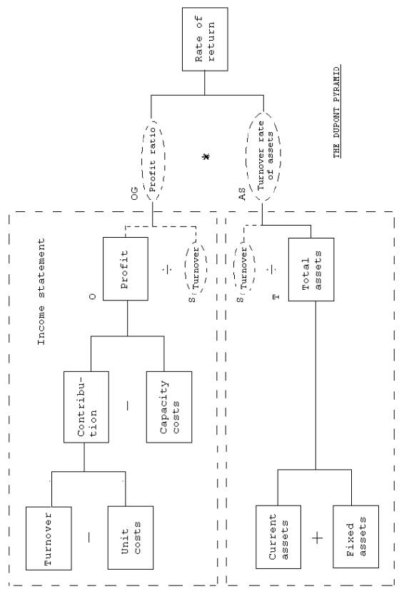
rowly defined for operations research purposes. - 49 - 13.2. Dupont pyramid Fig.
13.1. shows the Dupont pyramid containing the ratio, rate of return A. It will be seen that the Dupont
pyramid consists of two major components: Income Statement and Assets on the
basis of which the rate of return A by definition is computed as: O A = ¾¾¾ (192) T Equation
(192) can be transformed into O S A = ¾¾¾ ¾¾¾ (193) S T With
the definitions profit ratio OG and the turnover rate of assets AS, which are
both mathematical functions for operations research purposes, equation (193)
is given the form: A
= OG AS (194) In
connection with the computation of total assets T it is essential to note
that for accounting purposes it is difficult to determine the exact value of
the assets. How is, for example, the value of production machinery to be
valu- ed? The rate of return defined by equation (192) is thus a rough
measure of the financial efficiency of the production facilities. It
is pointed out that equation (194) has the same resulting informative con-
tents as equation (192). In equation (194) an extra variable in the form of
sales S has been put in. This ratio technique, which has been adopted by,
among others, Bela Gold, will be considered in greater detail in the follow-
ing pages. - 50 –
Figure 13.1 The
Dupont Pyramid - 51 - 13.2.1. Ratio mathematics, general For
the ratio U given by equation (195): y U = ¾¾¾ (195) x where
y and x are system variable and/or system state functions, financial or
physical, the general function given by equation (196) applies in the same
system:
y x1 xn xn+1
U = ¾¾¾
( ¾¾¾ - - - - ¾¾¾) ¾¾¾ (196) x1 x2 xn+1 x In
equation (196) xi for i = 1, -
- - -, n is an arbitrary quantity of system variable and/or system state
functions. If
we define the ratio G1
= y/x1, Gi = xi/xi+1 for i = 1, - - - , n and Gn = xn+1/x,
equation (196) may be given the equivalent form: U = G1 G2 G3 - - - - Gn (197) This
is exactly the ratio technique forming the basis of the computation of the
rate of return by the methods described in Section 12.2. (By the inserted va-
riable S in equation (193) or by the product method in equation (194)). A
look at Bela Gold's work on managerial ratios will show that equations (195),
(196) and (197) constitute the theoretical contents of Bela Gold's application
of ratios. It will be seen - 52 - that
exactly the assumptions underlying equation (196) are the reason why the
equation is not unique for a given system as regards the effect of the indi-
vidual ratios on U. Thus, these effects can only provide certain indications
as to states in the system under study. As
a result of the above comments on the lack of uniqueness of a number of
factors in a given development of a ratio, S, OG and AS are encircled by a
broken line in Fig. 13.1. The
above equations provide the theoretical background of the uncertainty found
in the literature on depiction of the Dupont pyramid. Thus, this pyramid is
often shown without the S, OG and AS areas encircled by broken lines. The
Dupont pyramid has a very simple memo-technical structure. This structure
consists of
Income Statment Assets Rate of return (ROI) The
Dupont pyramid is a kind of rough aid for analysis purposes rather than a
basic scientific figure with fundamental contents, cf. above. - 53 - Conclusion This
model of a company based on common accounting practrice presents all the most
applied functions of time giving management a picture of fundamental
characteristics in the company within accountancy, managerial economics, cash
flow, finance and physical resources. The business input parameters are di-
rectly available in the accountancy of the company. For
assessments of the soundness of cash flow released, two ratios have been
developed, interest relative and depreciation relative. The theoretical pro-
blem of Samuel Eilon,4-5 as
described in the introduction has been solved com- pletely. The
mathematical basis of Bela Gold's empirically applied ratio technique,7
has been discovered in order also to determine all the components in the
Dupont Pyramide as functions of time. As
a speciel powerfull result for management one may take the partial deriva-
tives of the funktions with the respect to the input data of accountancy and
also make the total differentials in order to make high efficient “what - if”
analysis. This implies also analysis of the effects of price elesticity of
markets. All
the functional expressions are implemented into the computer program MASI
proven in practice in more than 700 licensed installations in Scandinavia to
let the user get quick and deap insight into the dynamics of the company for
tactical and strategical planning purposes. The reader of this article may
ask for a licence to an english version under DOS, OS2 or WIN95 including a
manual (127 pages). - 54 - Acknowledgement Assosociate
Professor Mads Peter Soerensen, Department of Mathematical Model- ling, The
Technical University of Denmark, DK-2800 Lyngby, Denmark and profes- sor Jan
Mouritsen, Operation Management, Copenhagen Business School, Howitzvej 60,
DK-2000 Frederiksberg are gratefully acknowledged for illuminating
dis-cussions during the preparation of this manuscript. - 55
- BIBLIOGRAPHY
1. Ahlmark, Dan: Produkt - investering -
finansiering Ett bidrag till en teori foer foeretaget som ett produktcen- trerat finansiellt system. (292p) Handelshoegskolan i Stockholm Ekonomiska Forskningsinstitutet,
1974
2. Danielsson, Albert: Foeretagsekonomi. Begreppsbildning
och terminologie (79p) Studentlitteratur, Lund 1976 3. Danielsson,
Albert: Foeretagsekonomi
- en oeversikt (327p) Studentlitteratur, Lund 1975 4. Eilon,
Samuel & Cosmetatos, G.P.: A profitability model for tactical planning
OMEGA, Vol. 5, No. 6, pp673-688, 1977 5. Eilon,
S., Gold Bela, and Soesan J.:
Applied productivity analysis for industry (151p)
Pergamon Press, Oxford 1976 6. Forrester, Jay W.: Industrial
Dynamics (464p)
Cambridge, Mass.,M.I.T. Press 1977 7. Gold,
Bela:
Technological change. Economics, management and
environment (175p)
Pergamon Press, Oxford 1975 8.
Malmborg, Charles J.: Expected part delays as a secondary layout
criterion in
automated manufacturing systems App.
Math. Modelling 1997, 21: 301 - 313
Elsevier Science Inc. 1997 9.
Rappaport, Alfred:
Creating Shareholder Value (320p) Free
Press, Herts 1998 10. Segall,
R.S.:
Mathematical modelling of spatial price equilibrium for
multi commodity consumer flows of large markets
using variational inequalities App.
Math. Modelling, 1995, Vol 19, February
Elsevier Science Inc. 1995 |
|
|